CS 61B (Sp21) Notes 2, Data Structures

13. Asymptotics I

Our goal is to somehow characterize the runtimes of two functions. Characterization should be (1) simple and mathematically rigorous; and (2) demonstrate superiority of one over the other.

Asymptotic Analysis

Scaling Matters

In most cases, we care only about asymptotic behavior, i.e. what happens for very large $N$.

Algorithms which scale well (e.g. look like lines) have better asymptotic runtime behavior than algorithms that scale relatively poorly (e.g. look like parabolas). We’ll informally refer to the “shape” of a runtime function as its order of growth (will formalize soon).

• Often determines whether a problem can be solved at all.

Computing Worst Case Order of Growth (Tedious Approach)

• Construct a table of exact counts of all possible operations.

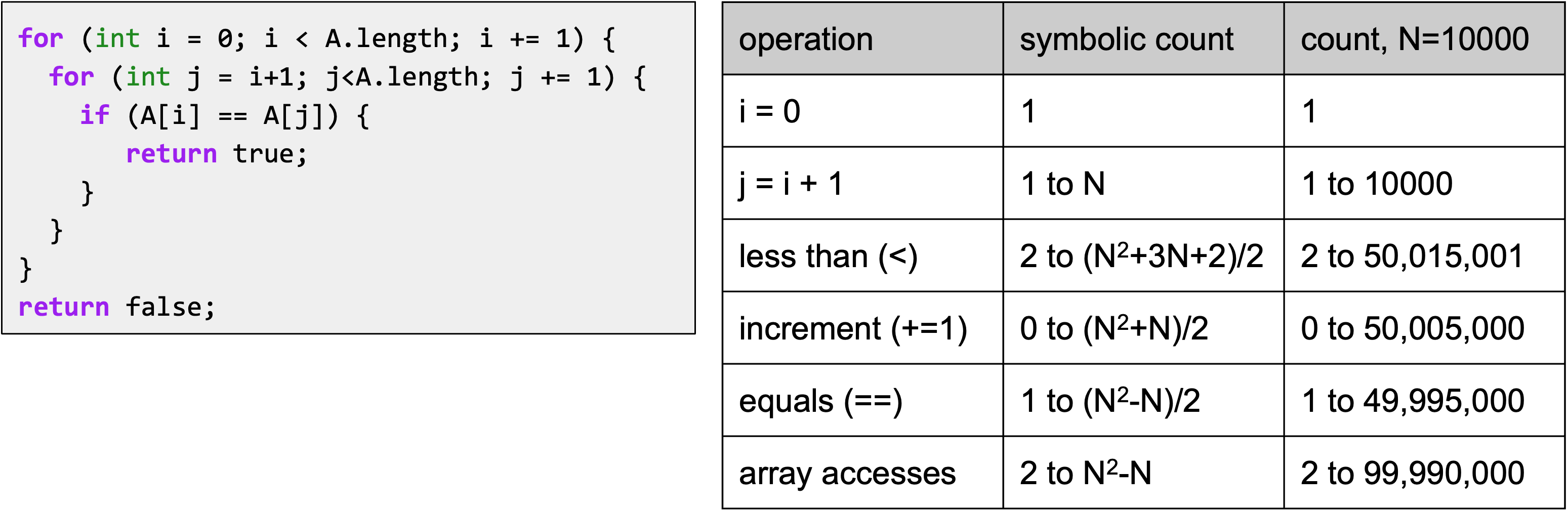
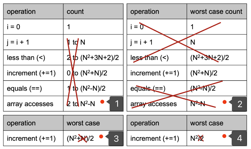
• Convert table into worst case order of growth using 4 simplifications:
  1. Only consider the worst case.
  2. Pick a representative operation (a.k.a. the cost model).
  3. Ignore lower order terms.
  4. Ignore multiplicative constants.

Computing Worst Case Order of Growth (Simplified Approach)

• Choose a representative operation to count (a.k.a. cost model).
• Figure out the order of growth for the count of the representative operation by either:
  • Making an exact count, then discarding the unnecessary pieces.
  • Using intuition and inspection to determine order of growth (only possible with lots of practice).

Asymptotic Notation

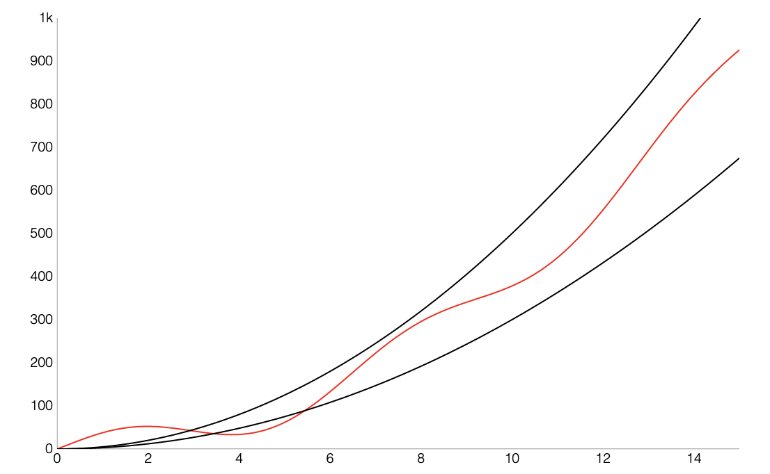
Big-Theta (a.k.a. Order of Growth)

For some function $R(N)$ with order of growth $f(N)$, we write that $R(N) \in \Theta(f(N))$. There exists some positive constants $k_1$, $k_2$ such that $k_1 \cdot f(N) \leq R(N) \leq k_2 \cdot f(N)$, for all values $N$ greater than some $N_0$ (a very large $N$).

Visualization

Big-O

$R(N) \in O(f(N))$ means that there exists positive constant $k_2$ such that $R(N) \leq k_2 \cdot f(N)$, for all values of $N$ greater than some $N_0$ (a very large $N$).

Visualization

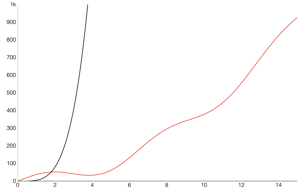
Whereas $\Theta$ can informally be thought of as something like “equals”, $O$ can be thought of as “less than or equal”.

Summary

Given a piece of code, we can express its runtime as a function $R(N)$, where $N$ is a property of the input of the function often representing the size of the input. Rather than finding the exact value of $R(N)$ , we only worry about finding the order of growth of $R(N)$. One approach (not universal):

• Choose a representative operation
• Let $C(N)$ be the count of how many times that operation occurs as a function of $N$
• Determine order of growth $f(N)$ for $C(N)$, i.e. $C(N) \in \Theta(f(N))$
• Often (but not always) we consider the worst case count
• If operation takes constant time, then $R(N) \in \Theta(f(N))$
• Can use $O$ as an alternative for $\Theta$. $O$ is used for upper bounds.

14. Disjoint Sets

Dynamic Connectivity Problem

Deriving the “Disjoint Sets” data structure for solving the “Dynamic Connectivity” problem. The Disjoint Sets data structure has two operations:

• connect(x, y): Connects x and y.
• isConnected(x, y): Returns true if x and y are connected. Connections can be transitive, i.e. they don’t need to be direct.

Goal: Design an efficient DisjointSets implementation.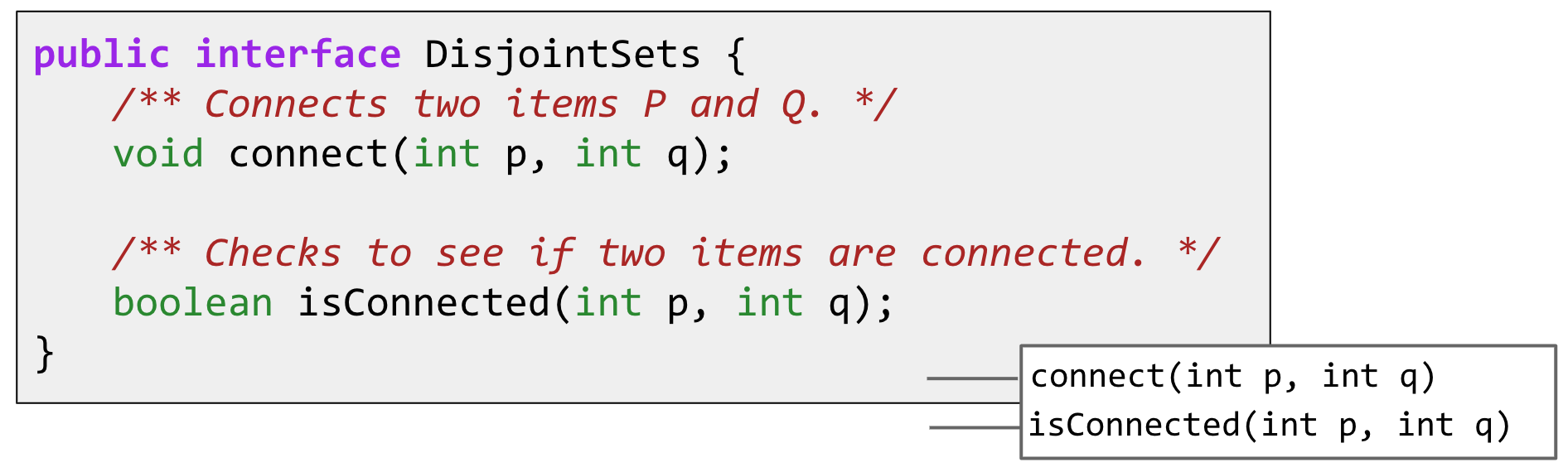

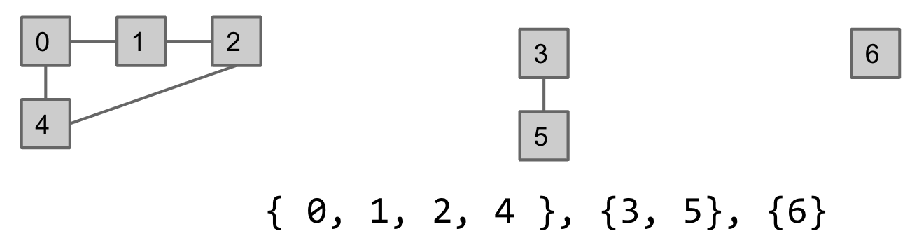
For each item, its connected component is the set of all items that are connected to that item. Model connectedness in terms of sets to keep track of which connected component each item belongs to.

Quick Find

Use an array of integers, where ith entry gives set number (a.k.a. “id”) of item i.

• connect(x, y): Change entries that equal id[x] to id[y].
• isConnected(x, y): Check if id[x] equals id[y].

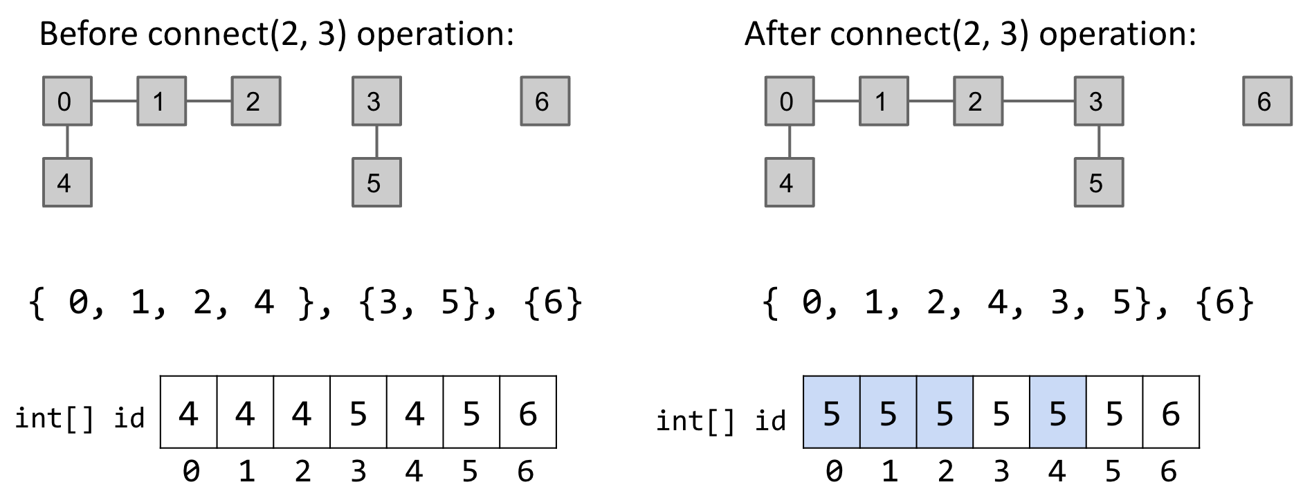
QuickFind is too slow for practical use: Connecting two items takes $N$ time.

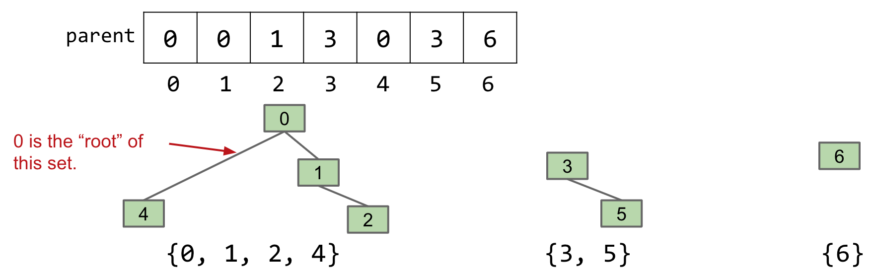
Quick Union

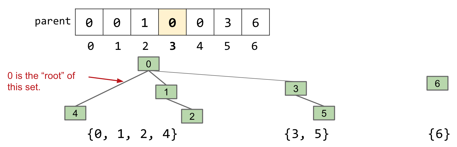
How could we change our set representation so that combining two sets into their union requires changing one value? Assign each item a parent (instead of an id). Results in a tree-like shape. Note: for root items, we have item’s parent as itself.

• connect(x, y): make root(x) into a child of root(y).
• isConnected(x, y): Check if root(x) equals root(y).

connect(5, 2): Make root(5) into a child of root(2)

Compared to QuickFind, we have to climb up a tree. Tree can get too tall and root(x) becomes expensive. Things would be fine if we just keep our tree balanced.

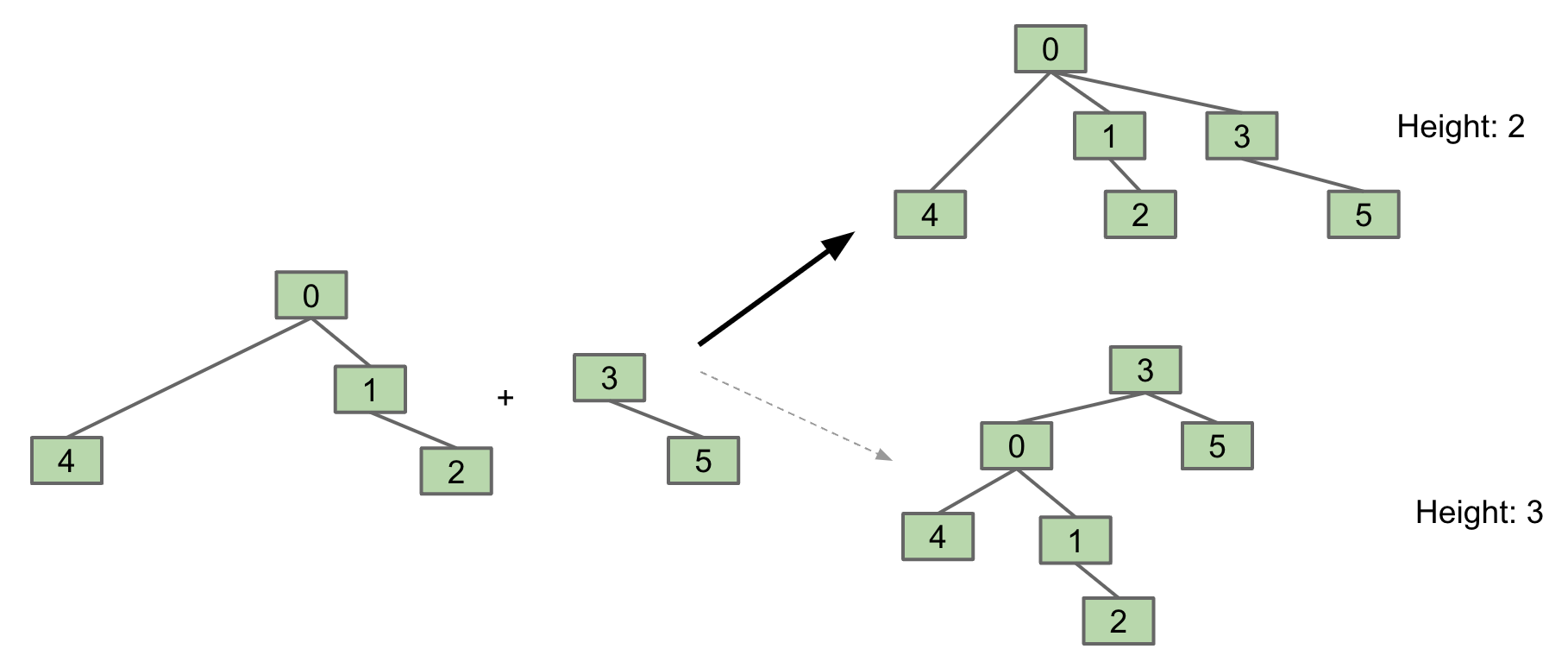
Weighted Quick Union

Modify quick-union to avoid tall trees. Track tree size (number of elements), and always link root of smaller tree to larger tree.

• connect(x, y): create a separate size array to keep track of sizes. make root(x) into a child of root(y), if size[root(x)] is smaller than size[root(y)], or vice versa.
• isConnected(x, y): Check if root(x) equals root(y).

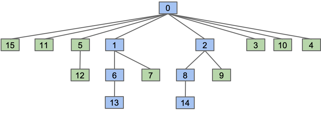
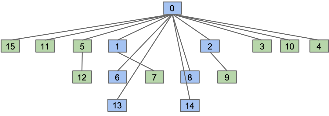
Path Compression

When we do isConnected(x, y), tie all nodes seen to the root.

16. ADTs, Sets, Maps, BSTs

Abstract Data Types

An Abstract Data Type (ADT) is defined only by its operations, not by its implementation. The built-in java.util package provides a number of useful:

• Interfaces: ADTs (List, Set, Map, etc.) and other stuff.
• Implementations: Concrete classes you can use.

List<Integer> L = new ArrayList<>();

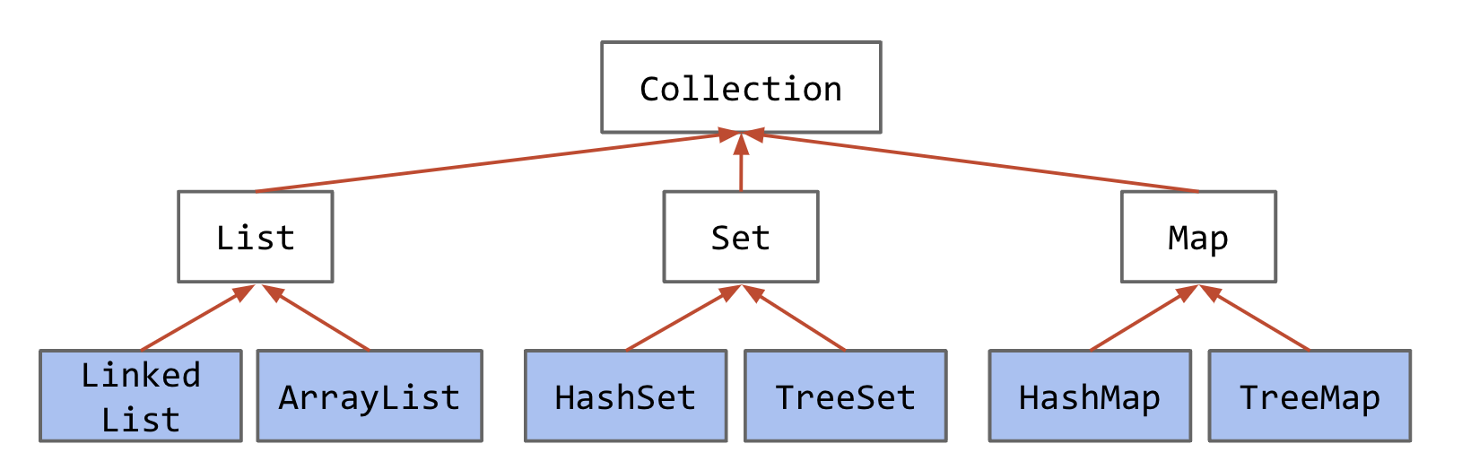Common interfaces in Java and their implementations

This lecture is about the basic ideas behind the TreeSet and TreeMap.

Binary Search Trees

Derivation

For the ordered linked list set implementation below, contains and add take worst case linear time, i.e. $\Theta(N)$. Fundamental Problem: Slow search, even though it’s in order.

In binary search, we know the list is sorted, so we can use this information to narrow our search. Applying binary search to a linked list might seem challenging at first. We need to traverse all the way to the middle to check the element there, which would take linear time.

However, we can optimize this process. One way is to keep a reference to the middle node. This allows us to reach the middle in constant time. Additionally, if we reverse the nodes’ pointers, we can traverse both the left and right halves of the list, effectively halving our runtime. We can further optimize by adding pointers to the middle of each recursive half like so.

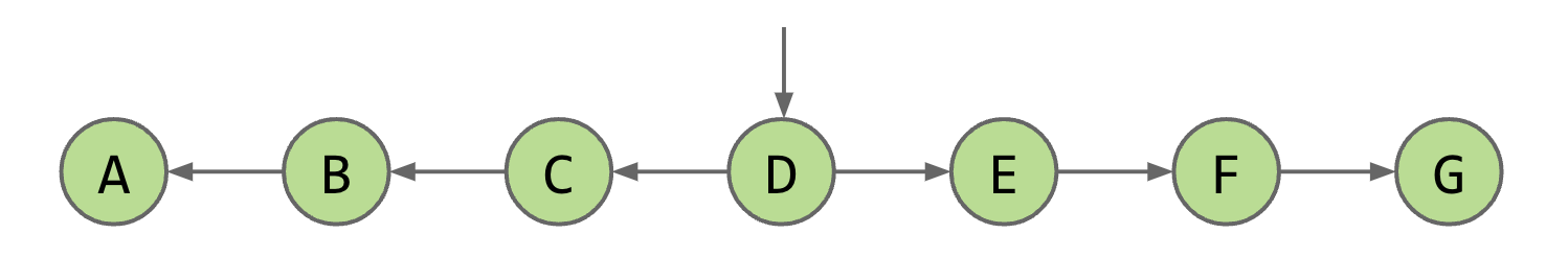A linked list with a middle pointer

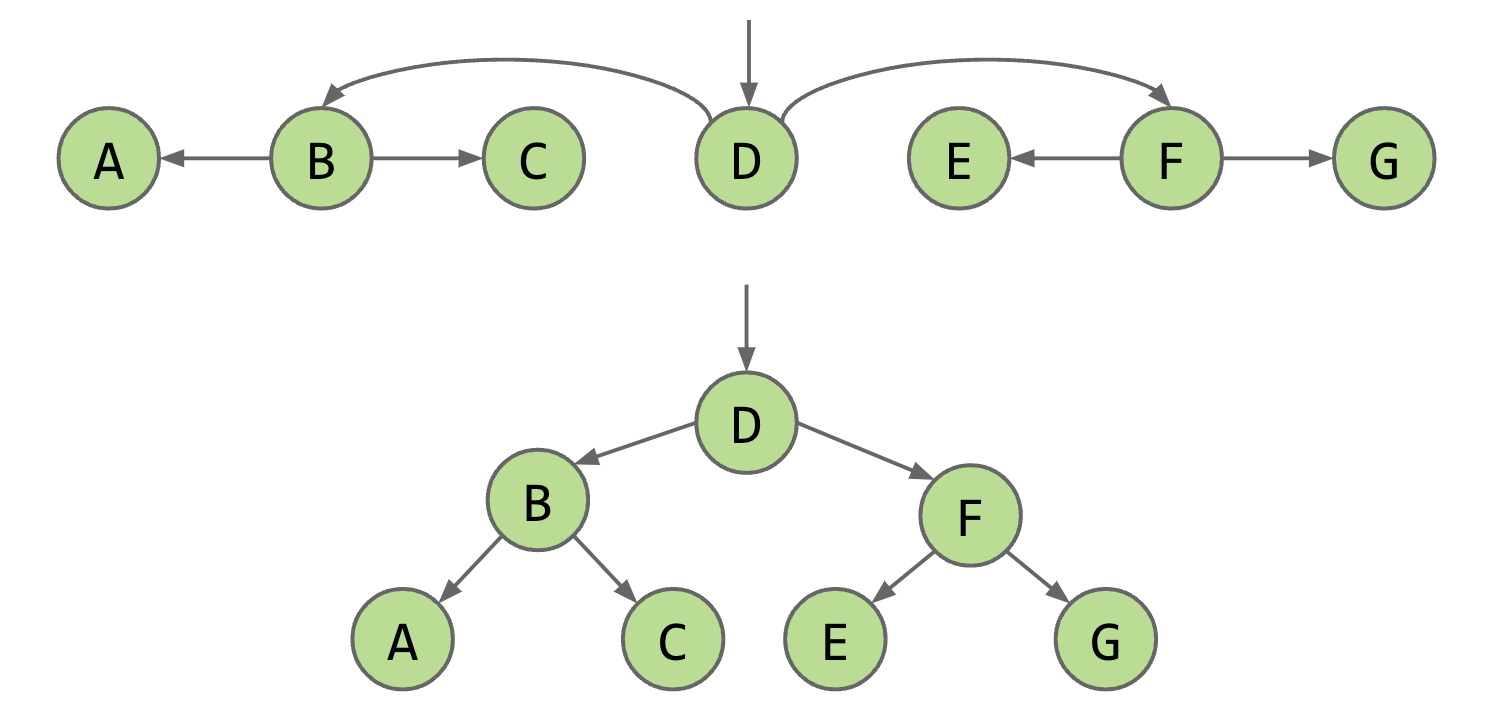A linked list with recursive middle pointers is a binary tree

Now, if you stretch this structure vertically, you will see a tree. This specific tree is called a binary tree because each juncture splits in 2.

BST Definition

A binary search tree is a rooted binary tree with the BST property, i.e., For every node X in the tree: every key in the left subtree is less than X’s key, and every key in the right subtree is greater than X’s key.

private class BST<Key> {
  private Key key;
  private BST left;
  private BST right;

  public BST(Key key, BST left, BST Right) {
    this.key = key;
    this.left = left;
    this.right = right;
  }

  public BST(Key key) {
    this.key = key;
  }
}

Contains

To find a searchKey in a BST, we employ binary search, which is made easy due to the BST property.

static BST find(BST T, Key sk) {
  if (T == null)
    return null;
  if (sk.equals(T.key))
    return T;
  else if (sk < T.key)
    return find(T.left, sk);
  else
    return find(T.right, sk);
}

The runtime to complete a search on a “bushy” BST in the worst case is $\Theta(\log N)$, where $N$ is the number of nodes.

Insert

We always insert at a leaf node.

static BST insert(BST T, Key ik) {
  if (T == null)
    return new BST(ik);
  if (ik < T.key)
    T.left = insert(T.left, ik);
  else if (ik > T.key)
    T.right = insert(T.right, ik);
  return T;
}

Deletion

Deleting from a binary tree is a little bit more complicated because whenever we delete, we need to make sure we reconstruct the tree and still maintain its BST property. Let’s break this problem down into three categories:

• the node we are trying to delete has no children
• has 1 child
• has 2 children

#####: Key with no Children We can just delete its parent pointer and the node will eventually be swept away by the garbage collector.

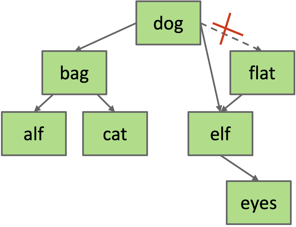
#####: Key with one Child The child maintains the BST property with the parent of the node because the property is recursive to the right and left subtrees. Therefore, we can just reassign the parent's child pointer to the node's child and the node will eventually be garbage collected.

Example: delete(“flat”)

#####: Key with two Children (Hibbard) If the node has two children, the process becomes a little more complicated because we can’t just assign one of the children to be the new root. This might break the BST property. Instead, we choose a new node to replace the deleted one. We know that the new node must:

• be > than everything in left subtree.
• be < than everything right subtree.

Example: delete(“dog”)

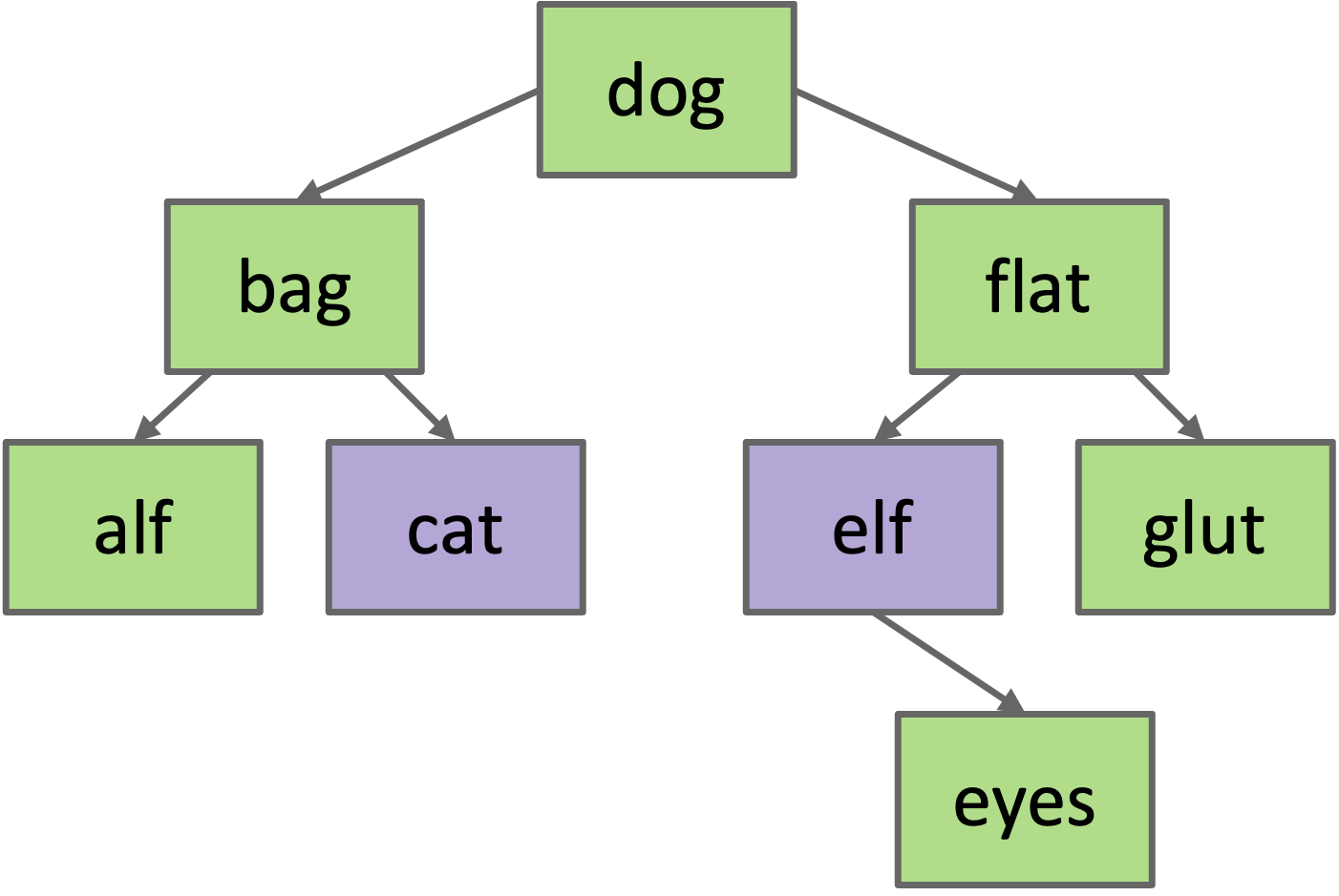
Choose either predecessor (cat, the right-most node in the left subtree) or successor (elf, the left-most node in the right subtree). Delete cat or elf, and stick new copy in the root position. This deletion guaranteed to be either case 1 or 2. This strategy is known as Hibbard deletion.

Sets and Maps

Set

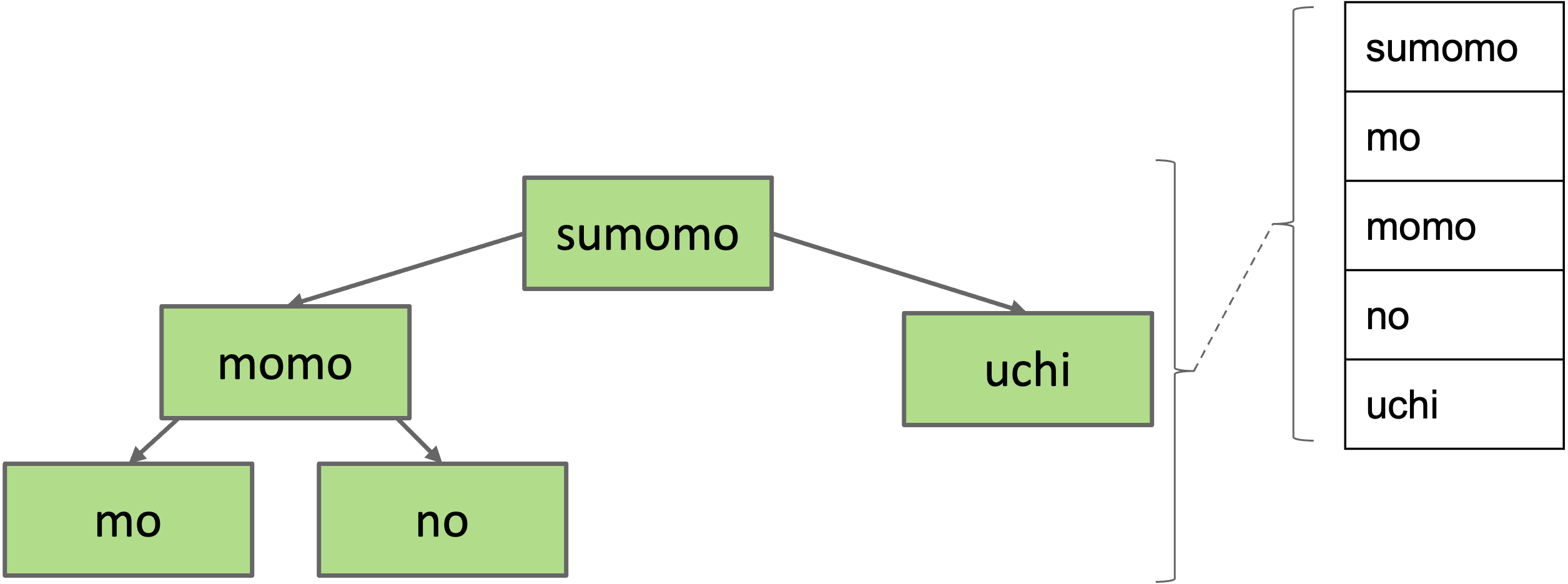
Can think of the BST below as representing a Set:

• {mo, no, sumomo, uchi, momo}

Map

To represent maps, just have each BST node store key/value pairs.

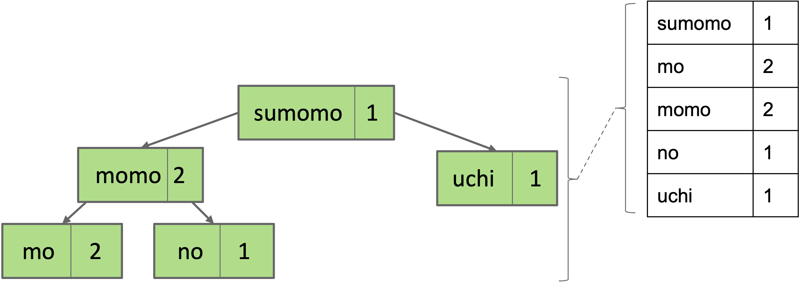
Note: No efficient way to look up by value.

• Example: Cannot find all the keys with value = 1 without iterating over ALL nodes. This is fine.

Summary

• Abstract data types (ADTs) are defined in terms of operations, not implementation.
  • Several useful ADTs: Disjoint Sets, Map, Set, List.
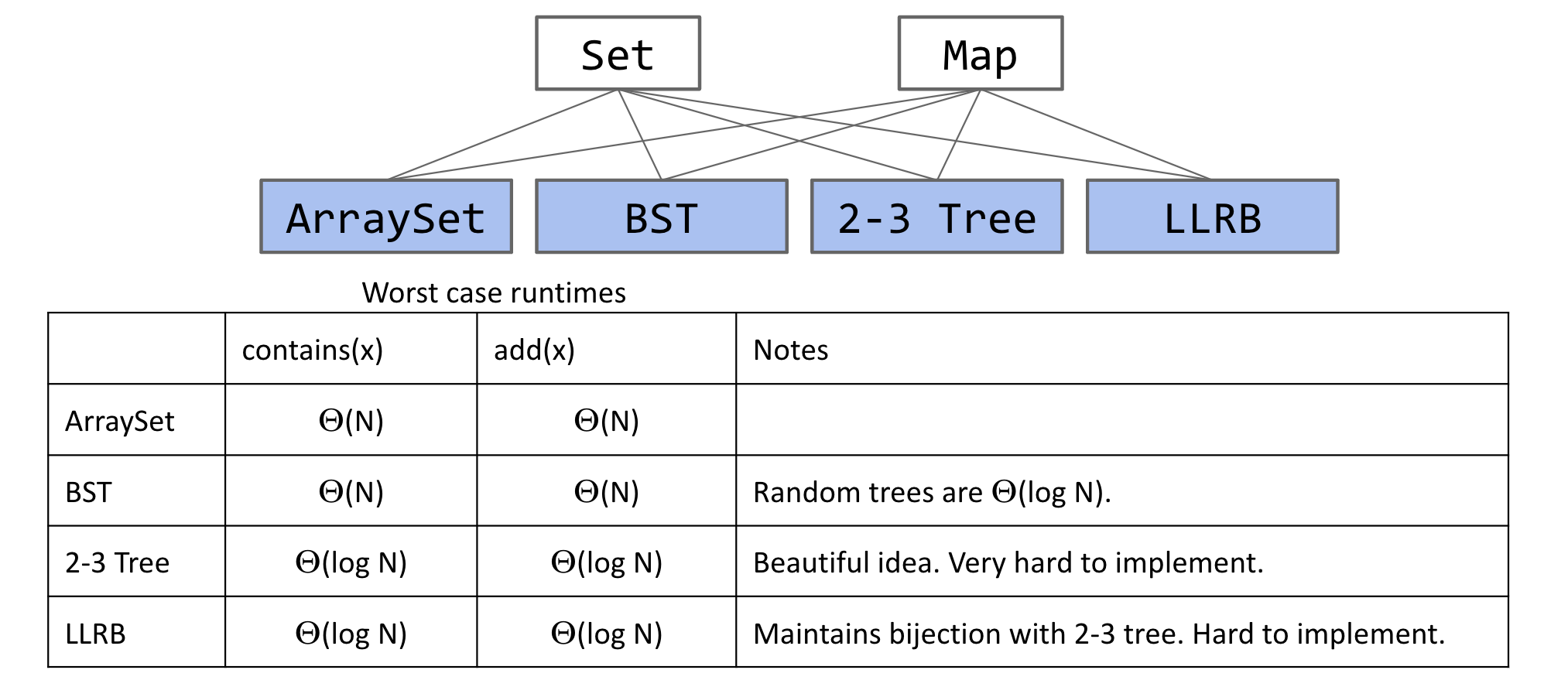
• Java provides Map, Set, List interfaces, along with several implementations.
• We’ve seen two ways to implement a Set (or Map):
  • ArraySet: $\Theta(N)$ operations in the worst case.
  • BST: $\Theta(\log N)$ operations if tree is balanced.
• BST Implementations:
  • Search and insert are straightforward (but insert is a little tricky).
  • Deletion is more challenging. Typical approach is “Hibbard deletion”.

Trees)

Binary Search Trees

BST Height

BST height is all four of these:

• $O(N)$.
• $\Theta(\log N)$ in the best case (“bushy”).
• $\Theta(N)$ in the worst case (“spindly”).
• $O(N^2)$.

Trees range from best-case “bushy” to worst-case “spindly”

Difference is dramatic!

Worst Case Performance

Height and Depth

• The depth of a node is how far it is from the root, e.g. depth(g) = 2.
• The height of a tree is the depth of its deepest leaf, e.g. height(T) = 4.

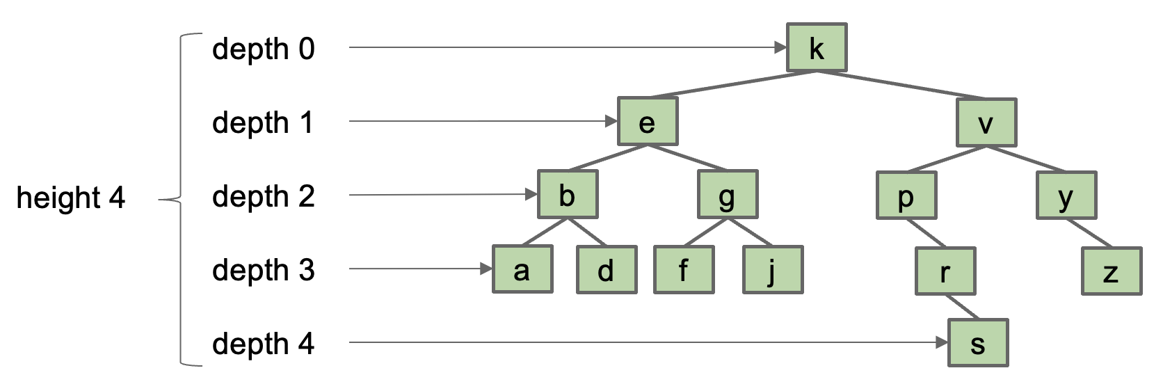
• The average depth of a tree is the average depth of a tree’s nodes.
  • (0x1 + 1x2 + 2x4 + 3x6 + 4x1)/(1+2+4+6+1) = 2.35

Runtime

• The height of a tree determines the worst case runtime to find a node.
  • Example: Worst case is contains(s), requires 5 comparisons (height + 1).
• The “average depth” determines the average case runtime to find a node.
  • Example: Average case is 3.35 comparisons (average depth + 1).

Nice Property

Random trees have $\Theta(\log N)$ average depth and height.

• Good news: BSTs have great performance if we insert items randomly. Performance is $\Theta(\log N)$ per operation.
• Bad News: We can’t always insert our items in a random order.

B-Trees

Splitting Juicy Nodes

Avoiding Imbalance through Overstuffing

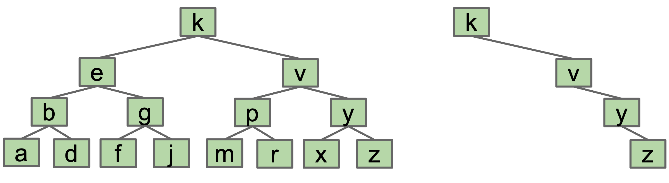
If we could simply avoid adding new leaves in our BST, the height would never increase.

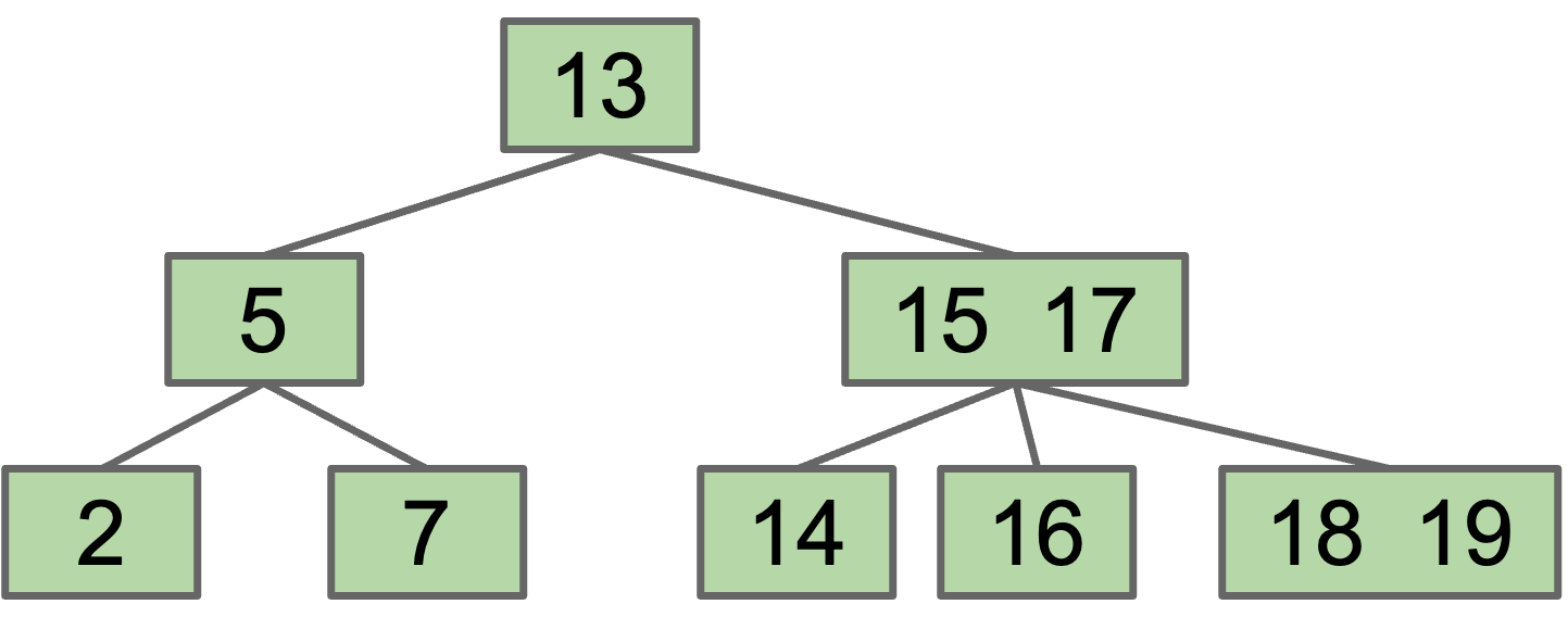
Instead of adding a new node upon insertion, we simply stack the new value into an existing leaf node at the appropriate location. Suppose we add 17, 18:

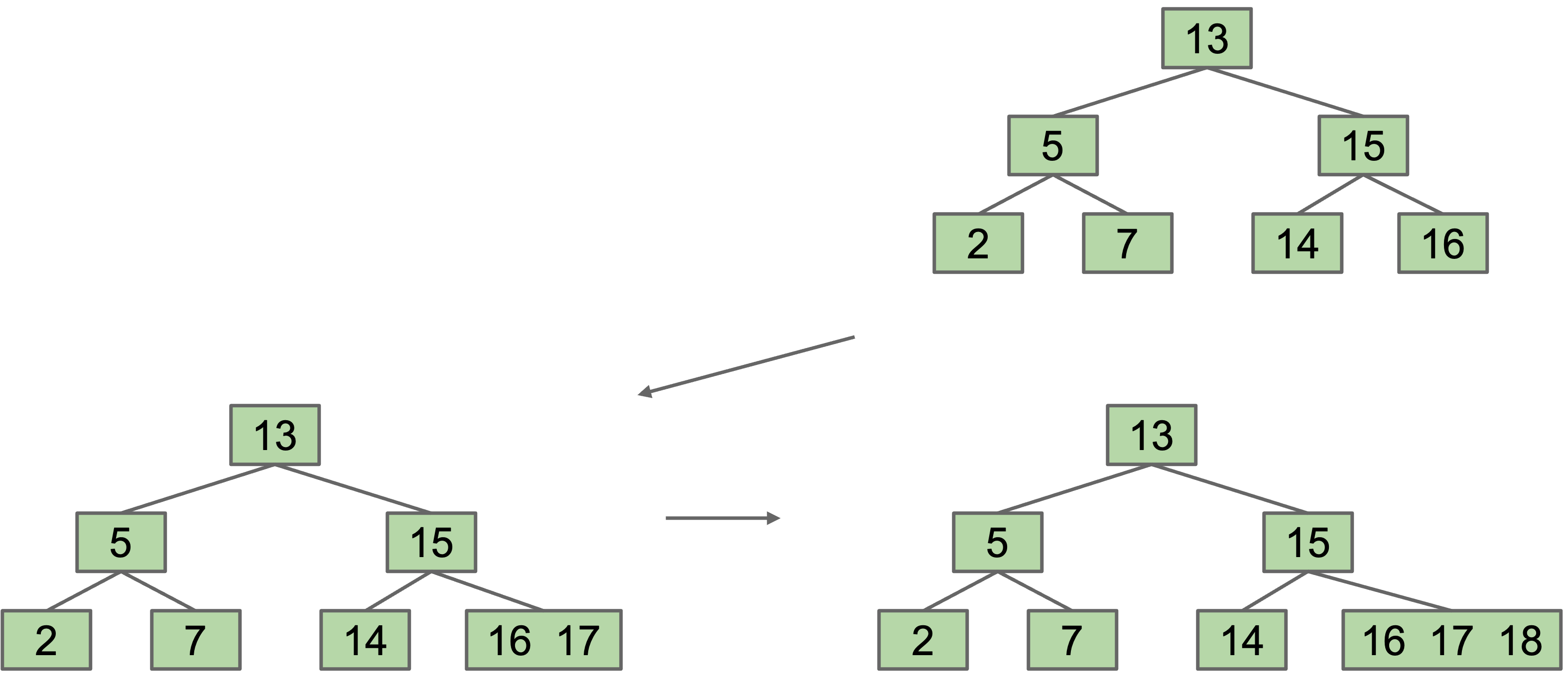Avoid new leaves by “overstuffing” the leaf nodes

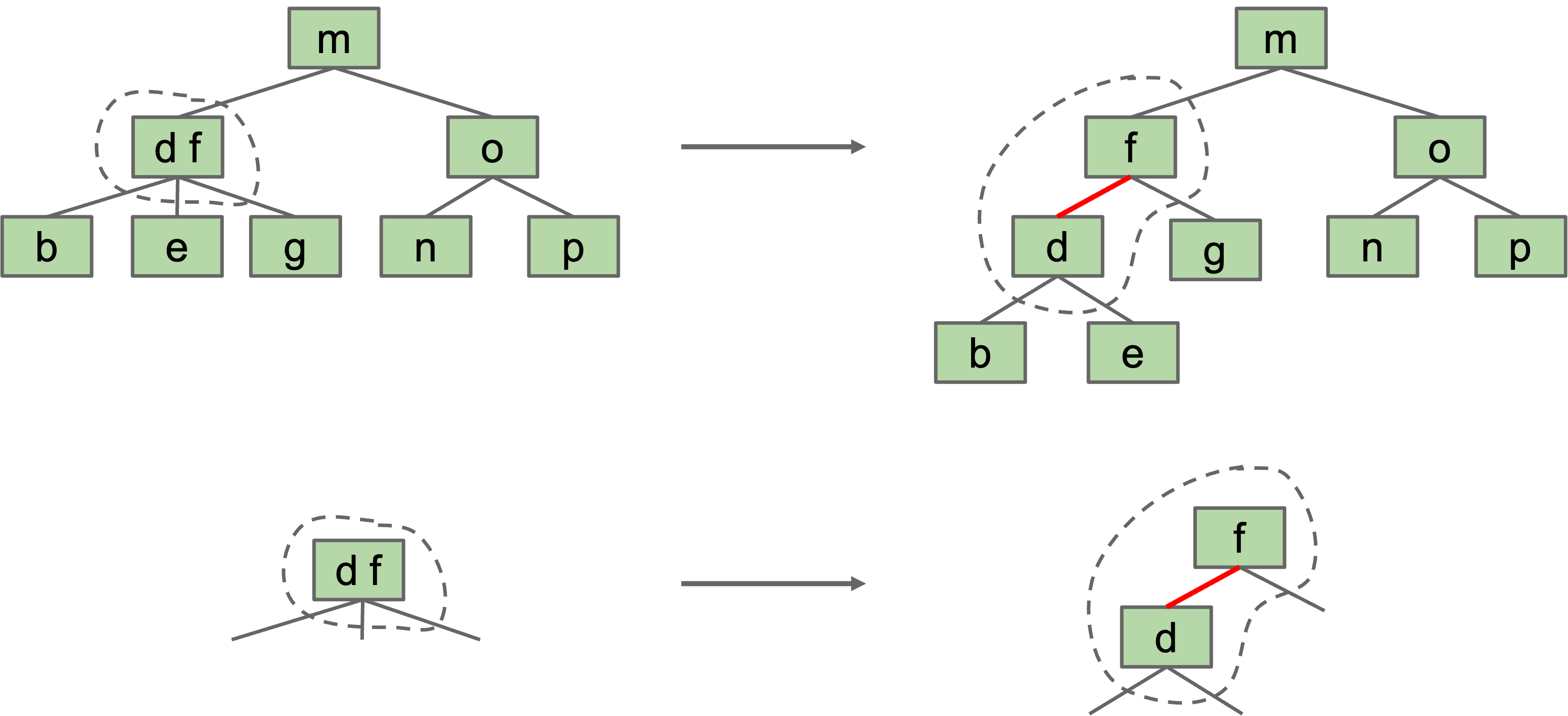
Moving Items Up

Height is balanced, but we have a new problem: Leaf nodes can get too juicy.

We can set a limit $L$ on the number of items, say $L=3$. If any node has more than $L$ items, give an item to parent. Which one? Let’s say (arbitrarily) the left-middle.

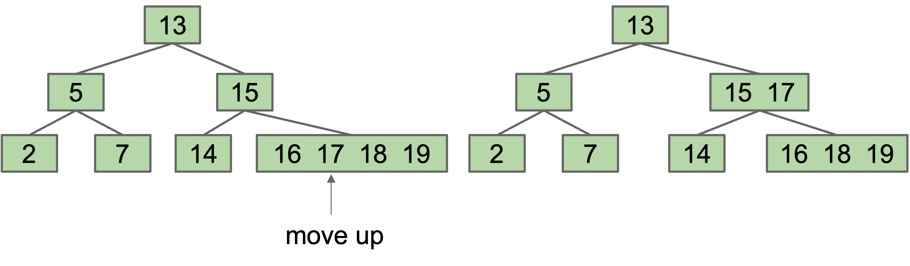Moving 17 from a leaf node to its parent

However, this runs into the issue that our binary search property is no longer preserved: 16 is to the right of 17. As such, we need a second fix: split the overstuffed node into ranges: $(-\infty,15)$, $(15, 17)$ and $(17, +\infty)$. Parent node now has three children.

Splitting the children of an overstuffed node

Chain Reaction Splitting

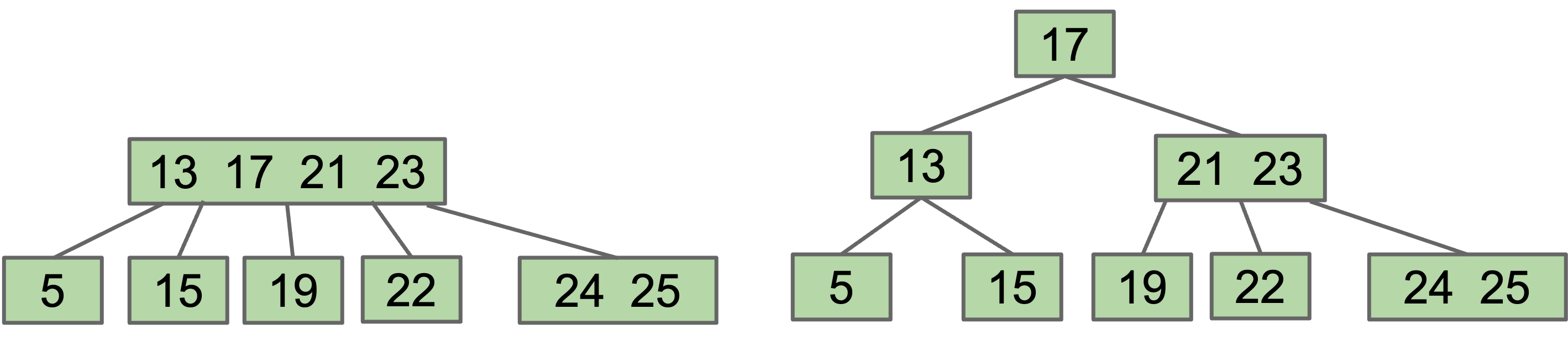
Suppose we add 25, 26:

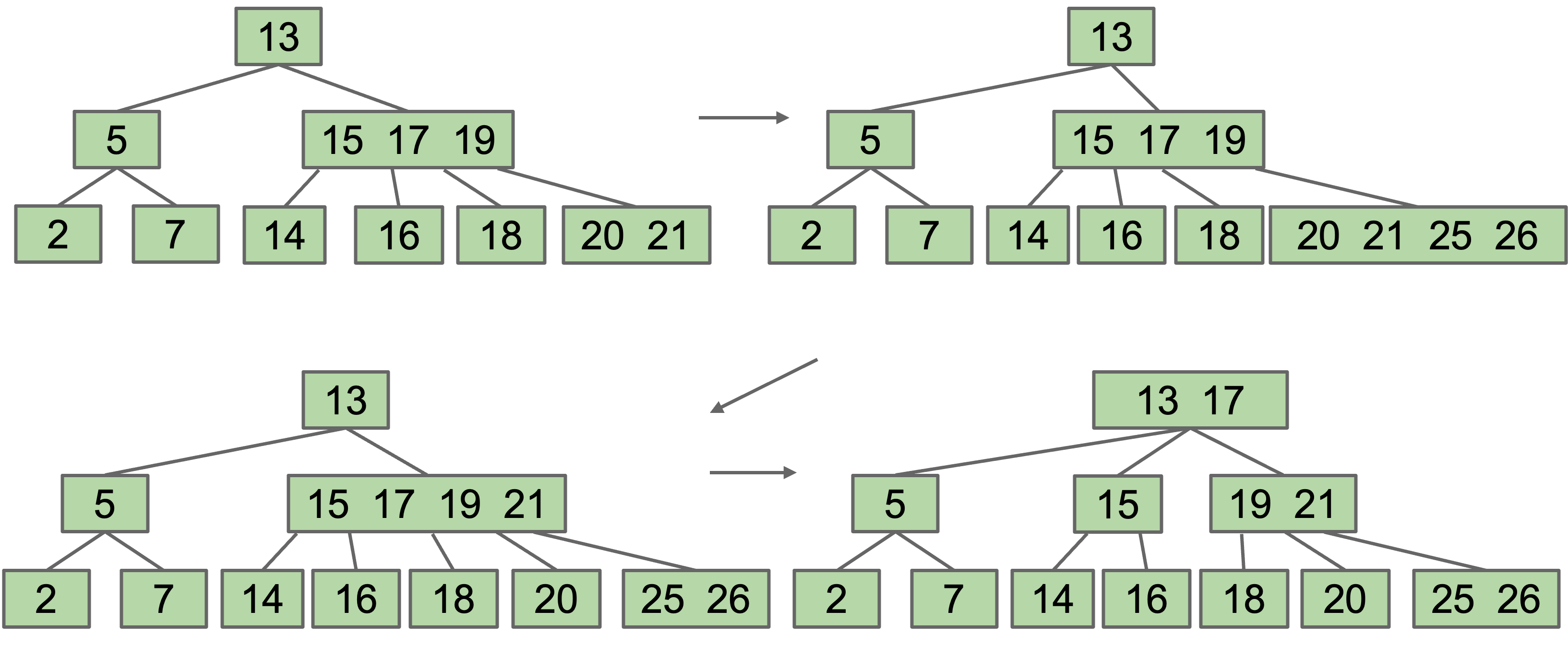
In the case when our root is above the limit, we are forced to increase the tree height.

B-Tree Terminology

The origin of “B-tree” has never been explained by the authors. As we shall see, “balanced,” “broad,” or “bushy” might apply. Others suggest that the “B” stands for Boeing. Because of his contributions, however, it seems appropriate to think of B-trees as “Bayer”-trees. – Douglas Corner (The Ubiquitous B-Tree)

Observe that our new splitting-tree data structure has perfect balance. If we split the root, every node is pushed down by one level. If we split a leaf or internal node, the height does not change. There is never a change that results in imbalance.

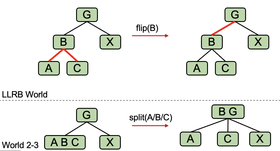
The real name for this data structure is a B-Tree. B-Trees with a limit of 3 items per node are also called 2-3-4 trees or 2-4 trees (a node can have 2, 3, or 4 children). Setting a limit of 2 items per node results in a 2-3 tree.

B-Trees are used mostly in two specific contexts:

• Small $L$ ($L=2$ or $L=3$):
  • Used as a conceptually simple balanced search tree (as today).
• $L$ is very large (say thousands).
  • Used in practice for databases and filesystems (i.e. systems with very large records).

B-Tree Invariants

Because of the way B-Trees are constructed, we get two nice invariants:

• All leaves must be the same distance from the root.
• A non-leaf node with $k$ items must have exactly $k+1$ children.

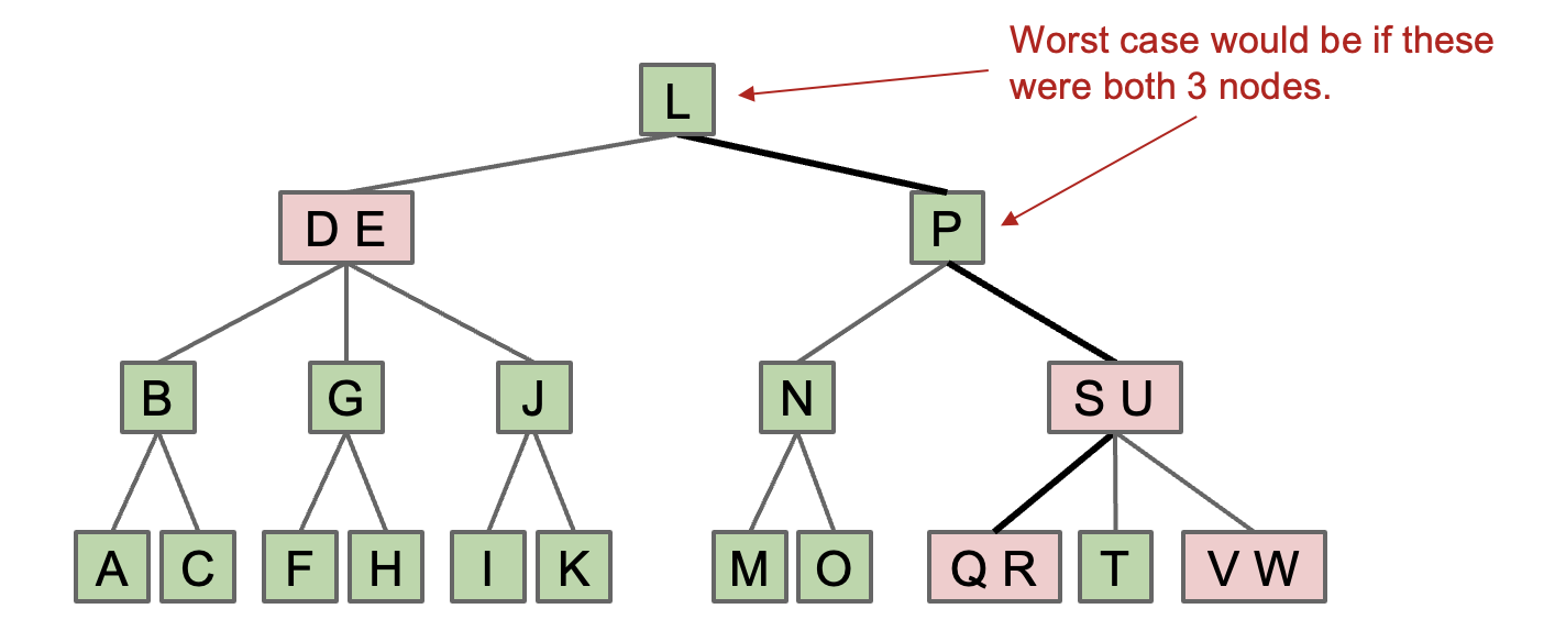
Worst Case Performance

Let $L$ be the maximum items per node. Based on our invariants, the maximum height must be somewhere between $\log_{L+1}(N)$ and $\log_2(N)$.

• Largest possible height is all non-leaf nodes have 1 item.

• Smallest possible height is all nodes have $L$ items.

Overall height is therefore $\Theta(\log N)$.

Runtime for contains

In the worst case, we have to examine up to $L$ items per node. We know that height is logarithmic, so the runtime of contains is bounded by $O(L \log N)$. Since $L$ is a constant, we can drop the multiplicative factor, resulting in a runtime of $O(\log N)$.

Runtime for add

A similar analysis can be done for add, except we have to consider the case in which we must split a leaf node. Since the height of the tree is $O(\log N)$, at worst, we do $\log N$ split operations (cascading from the leaf to the root). This simply adds an additive factor of $\log N$ to our runtime, which still results in an overall runtime of $O(\log N)$.

Summary

BSTs have best case height $\Theta(\log N)$, and worst case height $\Theta(N)$. B-Trees are a modification of the binary search tree that avoids $\Theta(N)$ worst case.

• Nodes may contain between 1 and $L$ items.
• contains works almost exactly like a normal BST.
• add works by adding items to existing leaf nodes.
  • If nodes are too full, they split.
• Resulting tree has perfect balance. Runtime for operations is $O(\log N)$.
• B-trees are more complex, but they can efficiently handle any insertion order.

Red Black Trees

Tree Rotation

BSTs

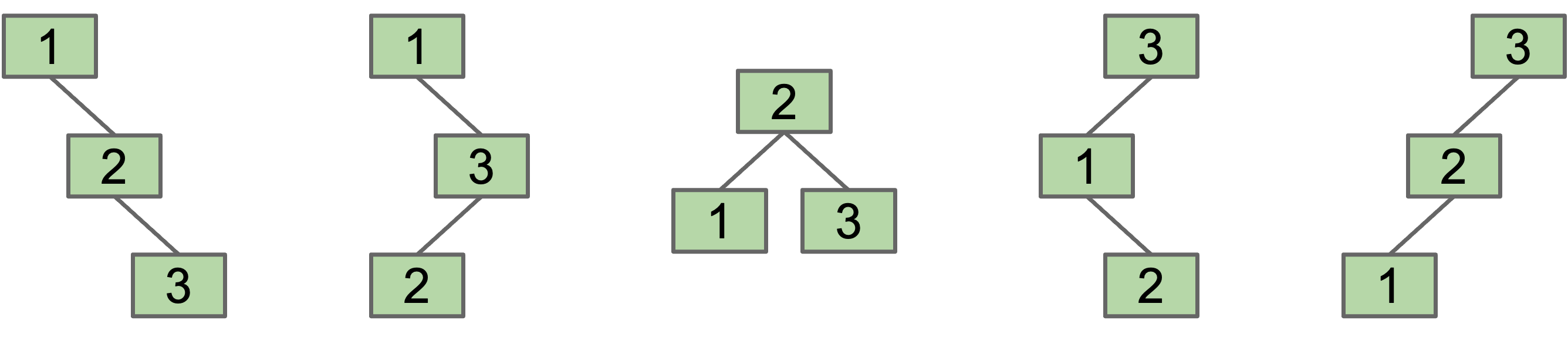
Suppose we have a BST with the numbers 1, 2, 3. Five possible BSTs.

• The specific BST you get is based on the insertion order.
• More generally, for $N$ items, there are Catalan(N) different BSTs.

Given any BST, it is possible to move to a different configuration using “rotation”.

• In general, can move from any configuration to any other in 2n - 6 rotations (see Rotation Distance, Triangulations, and Hyperbolic Geometry or Amy Liu).

Definition

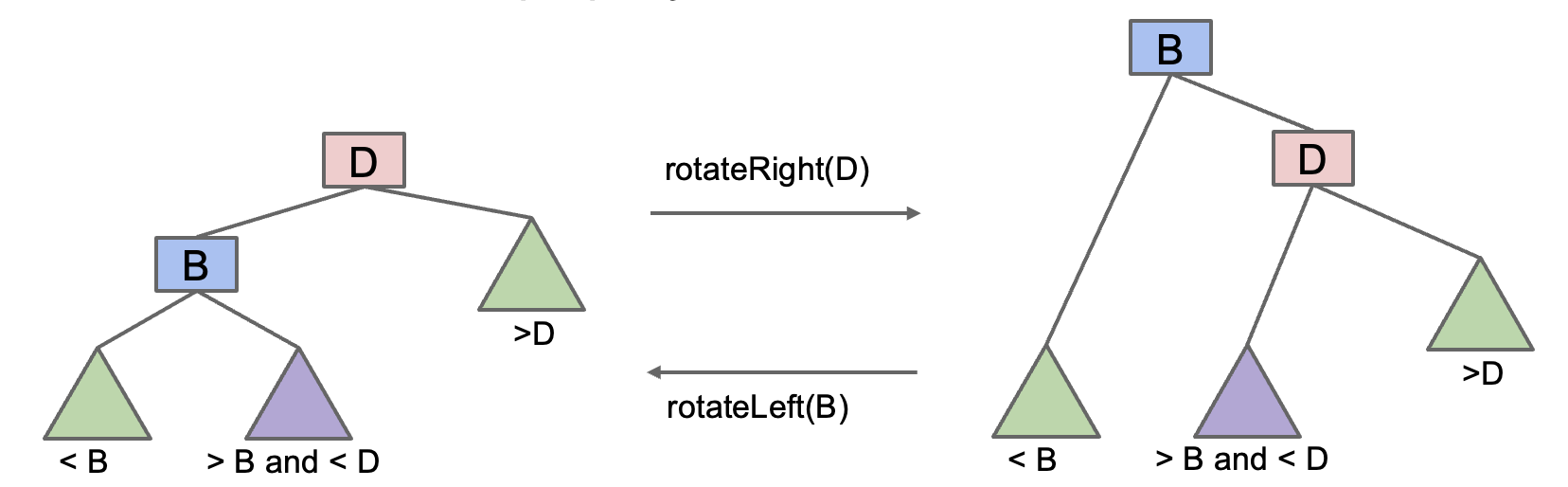
rotateLeft

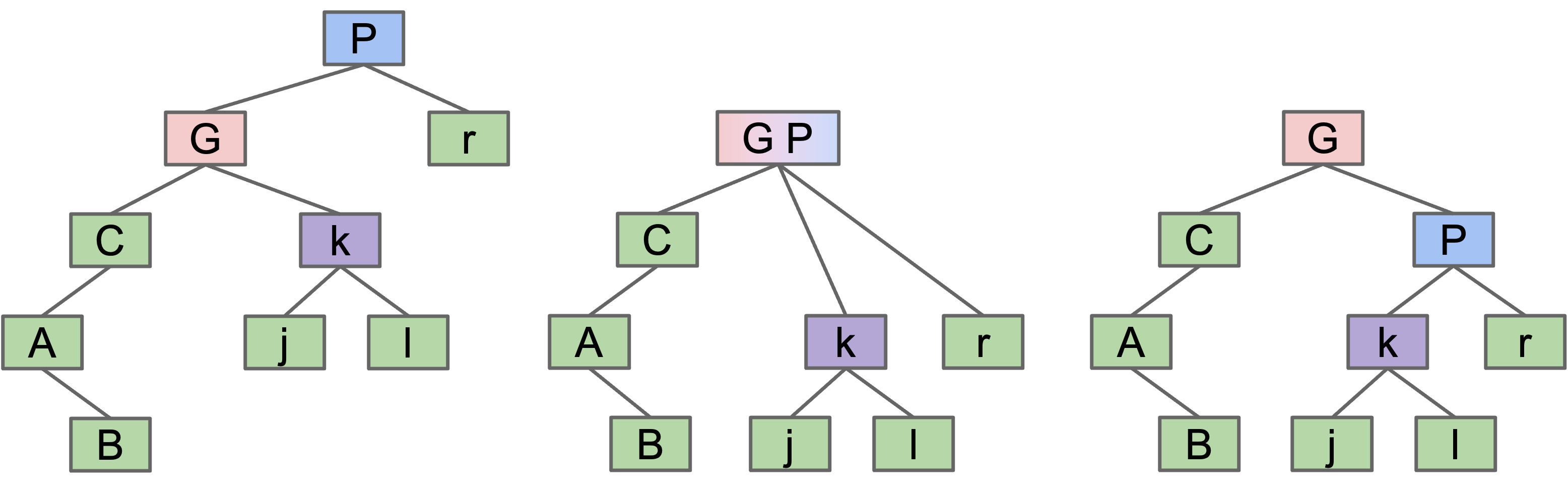
rotateLeft(G): Suppose x is the right child of G, make G the new left child of x.

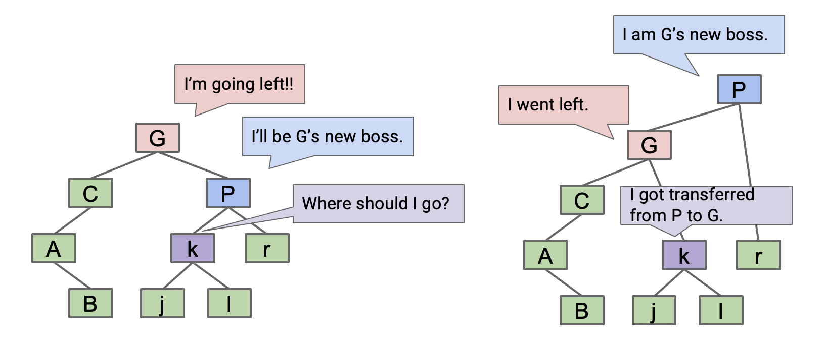
• Can think of as temporarily merging G and P, then sending G down and left.

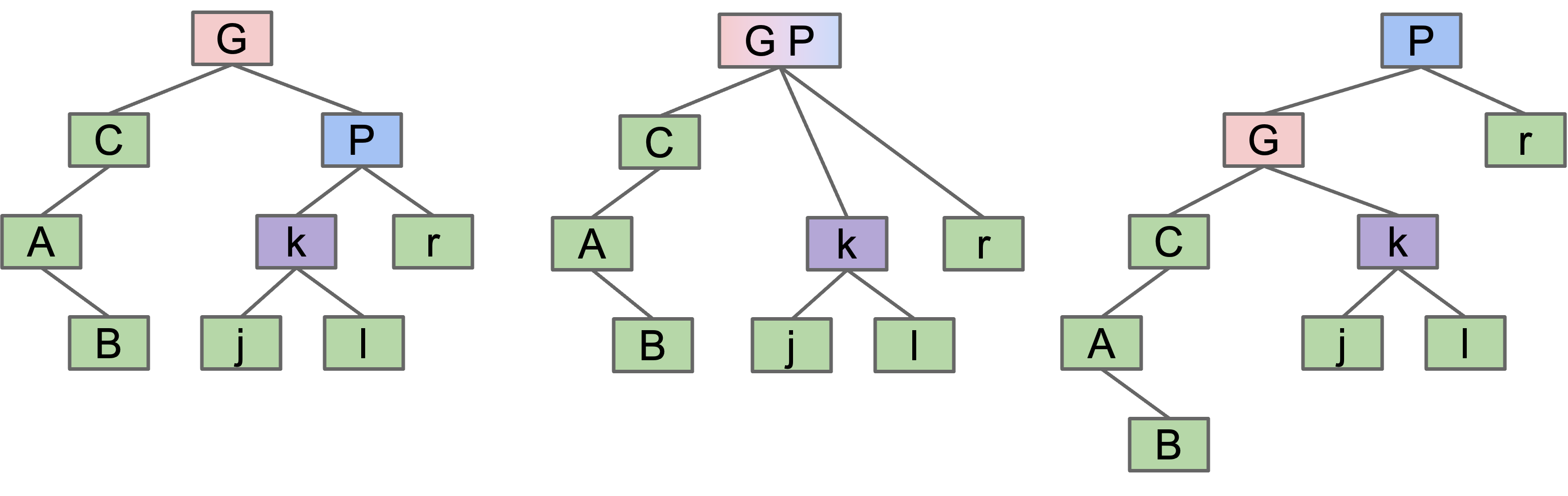
rotateRight

rotateRight(P): Suppose x is the left child of P, make P the new right child of x.

• Can think of as temporarily merging G and P, then sending P down and right.

Tree Balancing

Rotation:

• Can shorten (or lengthen) a tree.
• Preserves search tree property.

Rotation allows balancing of a BST in $O(N)$ moves.

Left Leaning Red-Black Trees (LLRBs)

Tree Isometry

2-3 trees always remain balanced, but they are very hard to implement. On the other hand, BSTs can be unbalanced, but are simple and intuitive. Is there a way to combine the best of two worlds? Why not create a tree that is implemented using a BST, but is structurally identical to a 2-3 tree and thus stays balanced?

Representing a 2-3 Tree as a BST

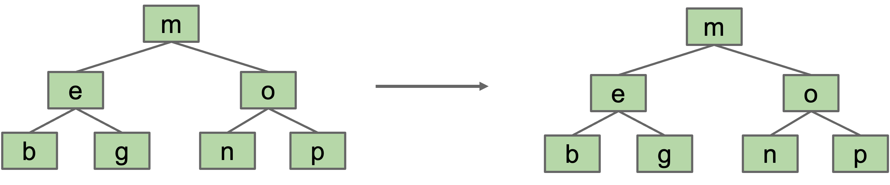
A 2-3 tree with only 2-nodes is trivial. BST is exactly the same.

Dealing with 3-Nodes

• Possibility 1: Create dummy “glue” nodes.

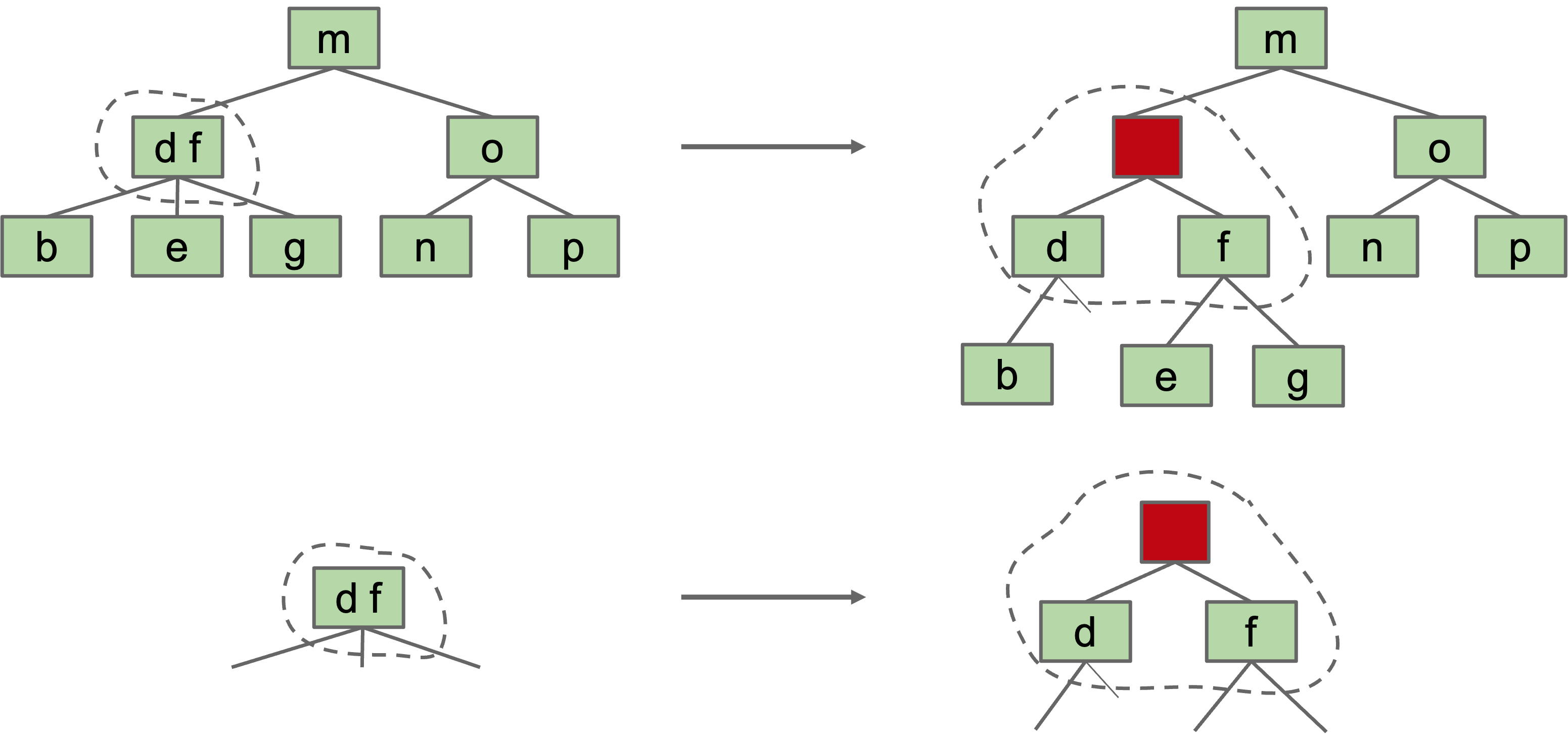Result is inelegant. Wasted link. Code will be ugly.

• Possibility 2: Create “glue” links with the smaller item off to the left.
  • For convenience, we’ll mark glue links as “red”.

Idea is commonly used in practice (e.g. java.util.TreeSet).

A BST with left glue links that represents a 2-3 tree is often called a “Left Leaning Red Black Binary Search Tree” or LLRB.

LLRB Properties

• Suppose we have a 2-3 tree of height H. The maximum height of the corresponding LLRB is
  • H (black) + H + 1 (red) = 2H + 1.

• No node has two red links [otherwise it’d be analogous to a 4 node, which are disallowed in 2-3 trees].
• Every path from root to null has same number of black links [because 2-3 trees have the same number of links to every leaf]. LLRBs are therefore balanced.

Maintaining Isometry with Rotations

When inserting into an LLRB tree, we always insert the new node with a red link to its parent node. This is because in a 2-3 tree, we are always inserting by adding to a leaf node, the color of the link we add should always be red.

But sometimes, inserting red links at certain places might lead to cases where we break one of the invariants of LLRBs. Below are three such cases where we need to perform certain tasks address in order to maintain the LLRB tree’s proper structure.

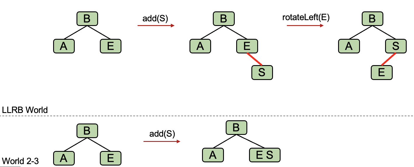
Case 1: Insertion on the Right

• If the left child is also a red link, go to case 3.
• Otherwise, Rotate E left.

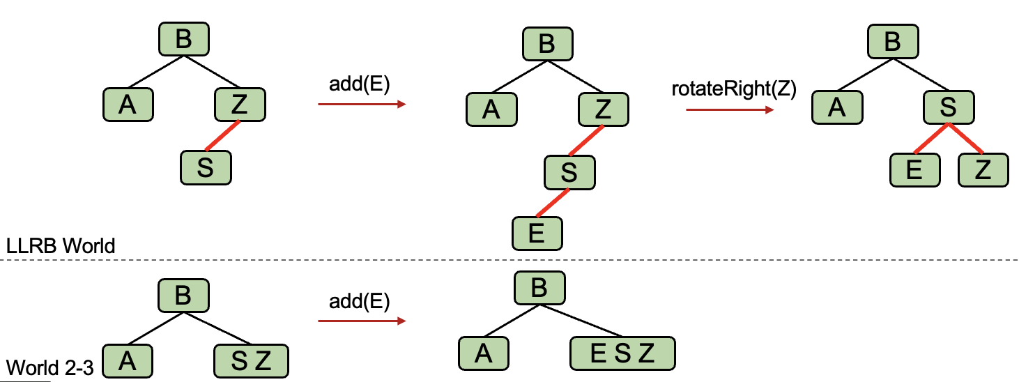
Case 2: Double Insertion on the Left

• Rotate Z right. Then go to case 3.

Case 3: Node has Two Red Children

• Flip the colors of all edges touching B.

Cascading operations

It is possible that a rotation or flip operation will cause an additional violation that needs fixing.

Runtime and Implementation

The runtime analysis for LLRBs is simple if you trust the 2-3 tree runtime.

• LLRB tree has height $O(\log N)$.
• contains is trivially $O(\log N)$.
• insert is $O(\log N)$.
  • $O(\log N)$ to add the new node.
  • $O(\log N)$ rotation and color flip operations per insert.

Hashing

Motivation

We’ve now seen several implementations of the Set (or Map) ADT.

Limits of Search Tree Based Sets:

• require items to be comparable
  • Could we somehow avoid the need for objects to be comparable?
• have excellent performance, but could maybe be better
  • Could we somehow do better than $\Theta(\log N)$?

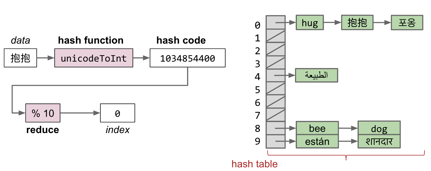
The Hash Table

• Data is converted by a hash function into an integer representation called a hash code.
• The hash code is then reduced to a valid index, usually using the modulus operator, e.g. 2348762878 % 10 = 8.

Hash Table Runtime

Suppose we have: an increasing number of buckets $M$, and an increasing number of items $N$. Even if items are spread out evenly, lists are of length $Q = \frac{N}{M}$. The contains(x) and add(x) have the worst case runtimes $\Theta(Q)$.

As long as $M = \Theta(N)$, then $O(\frac{N}{M}) = O(1)$. Resize when load factor $\frac{N}{M}$ exceeds some constant. If items are spread out nicely, you get $\Theta(1)$ average runtime. One example strategy: When $\frac{N}{M}$ is ≥ 1.5, then double $M$.

Heaps and PQs

Priority Queue

(Min) Priority Queue: Allowing tracking and removal of the smallest item in a priority queue. Useful if you want to keep track of the “smallest”, “largest”, “best” etc. seen so far.

public interface MinPQ<Item> {
    /** Adds the item to the priority queue. */
    public void add(Item x);
    /** Returns the smallest item in the priority queue. */
    public Item getSmallest();
    /** Removes the smallest item from the priority queue. */
    public Item removeSmallest();
    /** Returns the size of the priority queue. */
    public int size();
}

Heaps

Heap Structure

BSTs would work, but need to be kept bushy and duplicates are awkward.

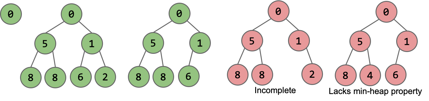
Binary min-heap: Binary tree that is complete and obeys min-heap property.

• Min-heap: Every node is less than or equal to both of its children.
• Complete: Missing items (if any) only at the bottom level, all nodes are as far left as possible.

Add

Algorithm for add(x): to maintain the completeness, the natural thought is to place x in the leftmost empty spot on the lowest level. However, this doesn’t guarantee the min-heap property, so further adjustments are needed.

swim: Continually compare x with its parent. If x is smaller, swap it with the parent. Repeat this process until x is in the right position.

Delete

Algorithm for removeSmallest(): to maintain the completeness of the structure, the intuitive approach is to swap the root node with the node at the end, then remove it. However, this doesn’t guarantee the min-heap property, so further adjustments are needed.

sink: Continually compare x with its left and right nodes. Swap x with the smaller of the two nodes. Repeat this process until x is in the right position.

Heap Operations Summary

• getSmallest() - return the item in the root node.
• add(x) - place the new employee in the last position, and promote as high as possible.
• removeSmallest() - assassinate the president (of the company), promote the rightmost person in the company to president. Then demote repeatedly, always taking the ‘better’ successor.

Tree Representation

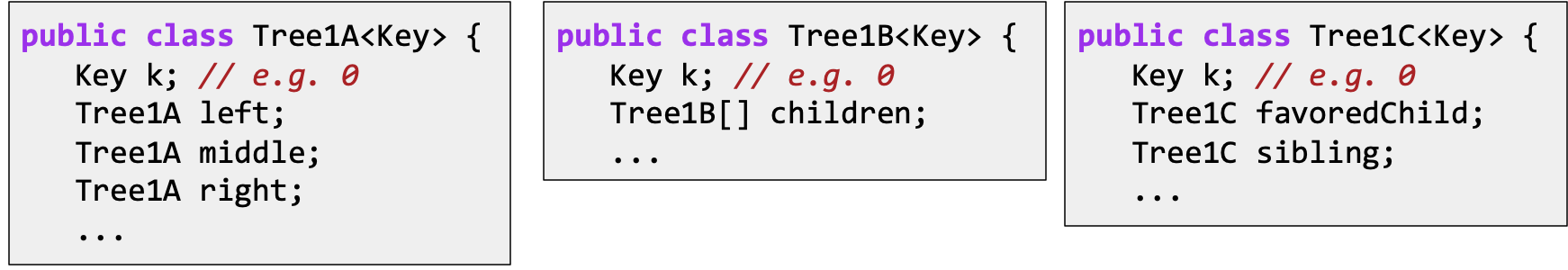
How do we Represent a Tree in Java?

####c Create mapping from node to children.

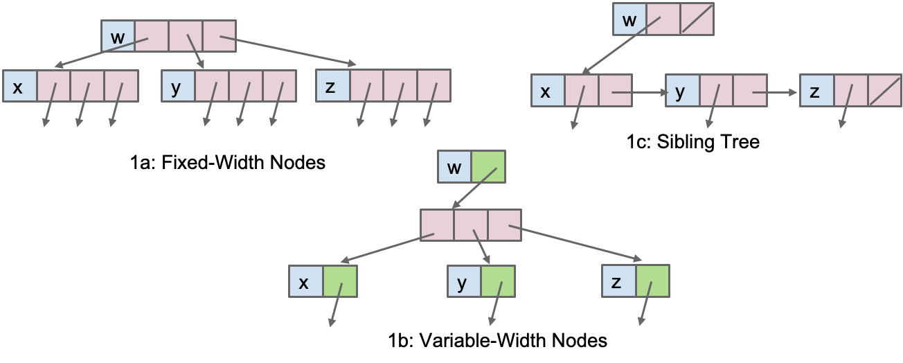
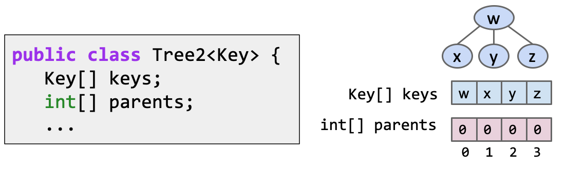
#### Store keys in an array. Store parentIDs in an array.

• Similar to what we did with disjointSets.

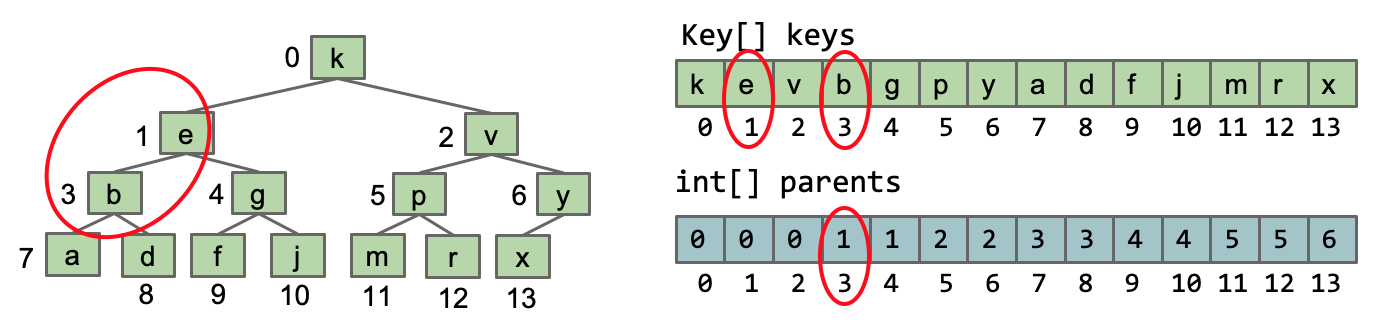
A more complex example：

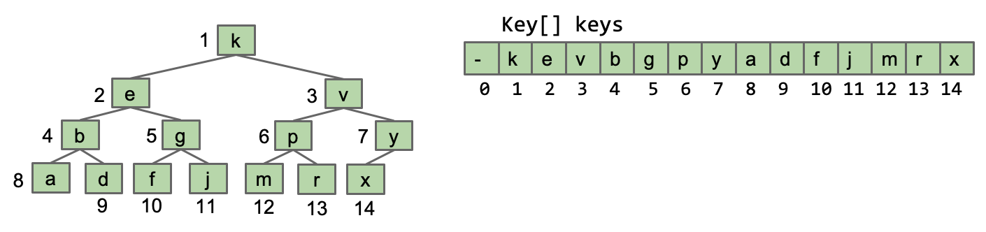
#### Store keys in an array. Don’t store structure anywhere.

In Approach2, we observe that when numbering a binary tree in the order of level traversal, if the tree has the property of being complete, there is a pattern between the parent and child node numbers: the parent number corresponding to the node number $k$ is $\frac{k-1}{2}$.

Further, if we leave the 0th position empty, the following patterns emerge:

• leftChild(k) $= 2k$
• rightChild(k) $= 2k + 1$
• parent(k) = $\frac{k}{2}$

Tree and Graph Traversals

Trees

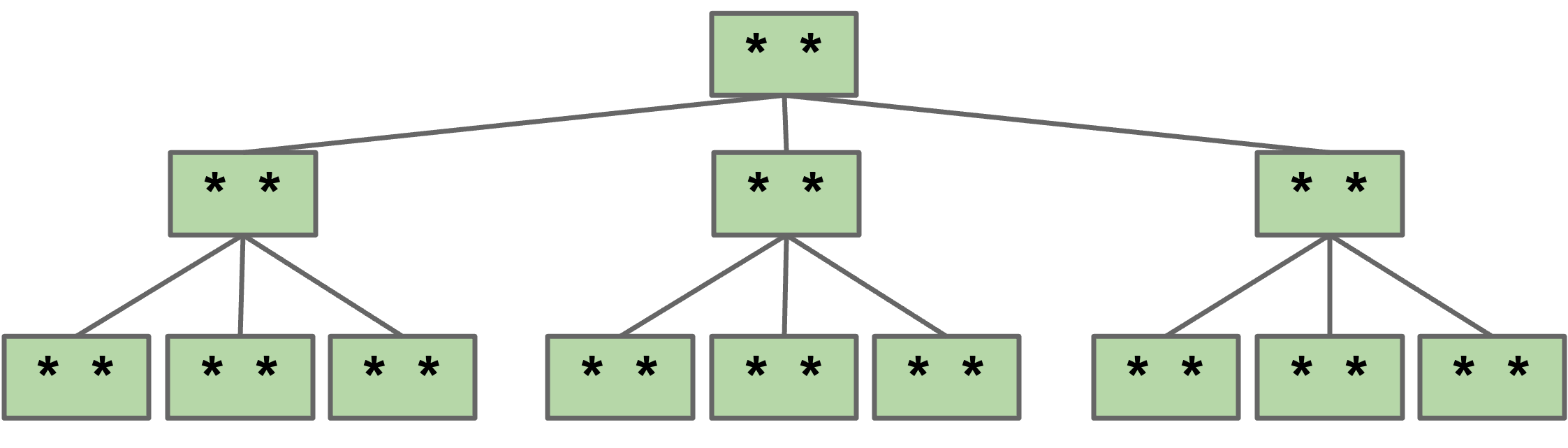
Tree Definition

A tree consists of a set of nodes and a set of edges that connect those nodes, where there is exactly one path between any two nodes.

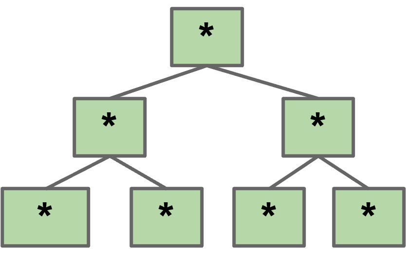
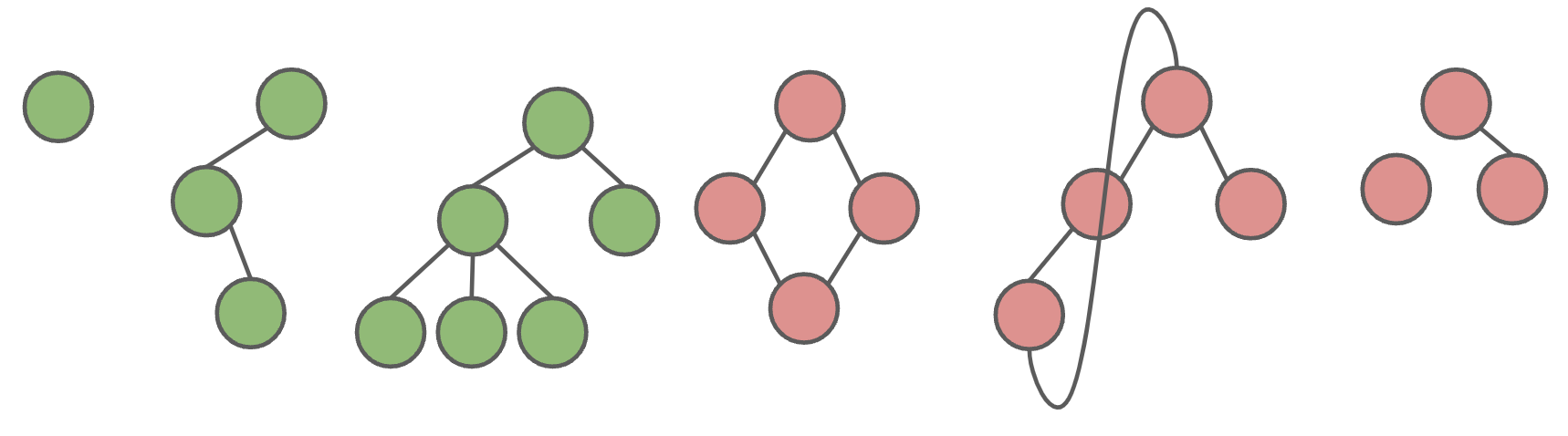Green structures below are trees. Pink ones are not.

Tree Traversals

Sometimes you want to iterate over a tree. What one might call “tree iteration” is actually called “tree traversal”. Unlike lists, there are many orders in which we might visit the nodes.

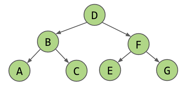
Level Order

• DBFACEG

Depth First Traversals

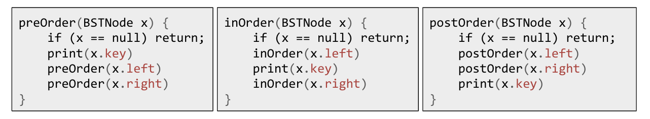DBACFEG | ABCDEFG | ACBEGFD

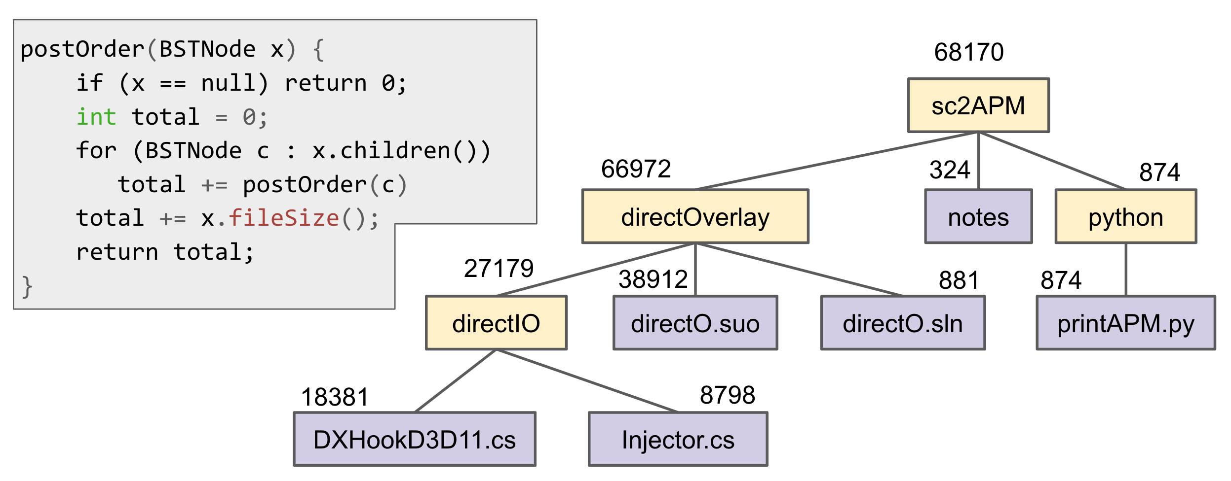
Usefulness of Tree Traversals

Preorder Traversal for printing directory listing

Postorder Traversal for gathering file sizes

Graphs

Graph Definition

Trees are fantastic for representing strict hierarchical relationships. But not every relationship is hierarchical. A graph consists of a set of nodes and a set of zero or more edges, each of which connects two nodes. Note, all trees are graphs.

A simple graph is a graph with:

• No edges that connect a vertex to itself, i.e. no “length 1 loops”.
• No two edges that connect the same vertices, i.e. no “parallel edges”.

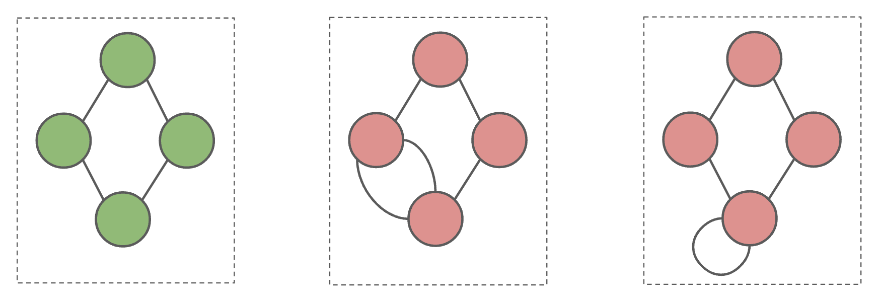Green graph below is simple, pink graphs are not.

In 61B, unless otherwise explicitly stated, all graphs will be simple.

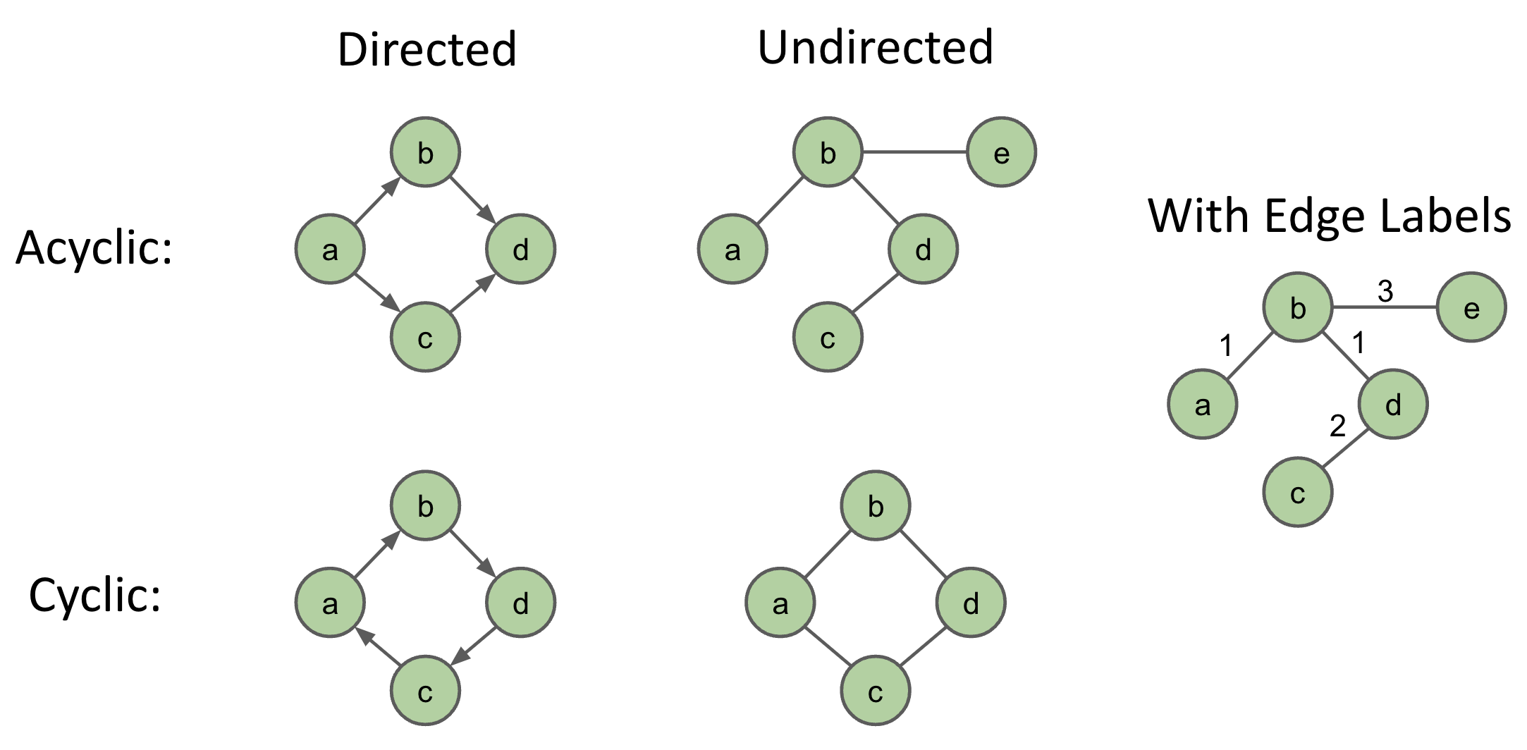
Graph Types

Graph Problems

Some well known graph problems and their common names:

• s-t Path. Is there a path between vertices s and t?
• Connectivity. Is the graph connected, i.e. is there a path between all vertices?
• Biconnectivity. Is there a vertex whose removal disconnects the graph?
• Shortest s-t Path. What is the shortest path between vertices s and t?
• Cycle Detection. Does the graph contain any cycles?
• Euler Tour. Is there a cycle that uses every edge exactly once?
• Hamilton Tour. Is there a cycle that uses every vertex exactly once?
• Planarity. Can you draw the graph on paper with no crossing edges?
• Isomorphism. Are two graphs isomorphic (the same graph in disguise)?

Graph Traversals

Motivation: s-t Connectivity

Let’s solve a classic graph problem called the s-t connectivity problem. Given source vertex s and a target vertex t, is there a path between s and t?

A path is a sequence of vertices connected by edges.

One possible recursive algorithm for connected(s, t).

def connected(s, t):
    if s == t:
        return True
    for v in neighbors_of(s):
        if connected(v, t):
            return True
    return False

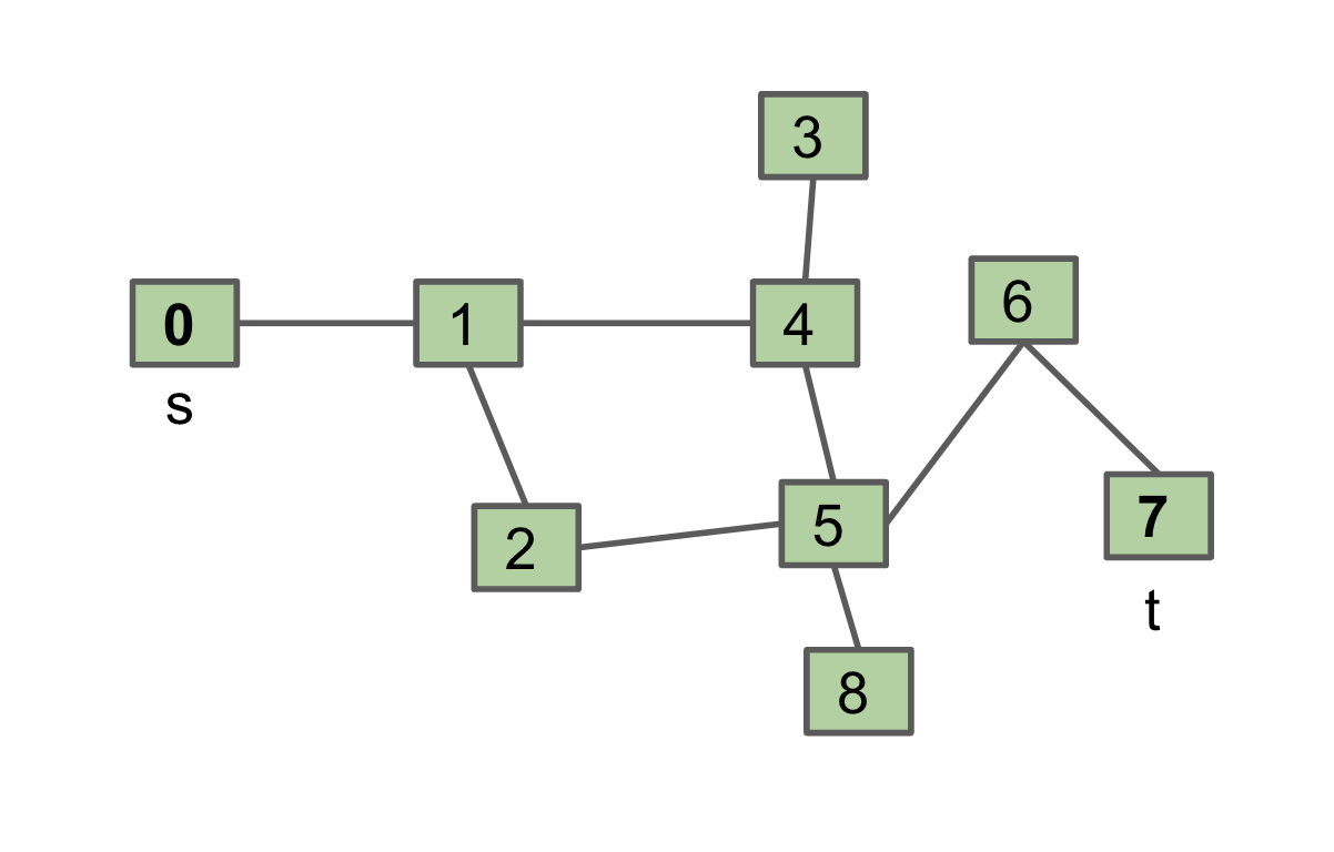
What is wrong with it? Can get caught in an infinite loop. Example:

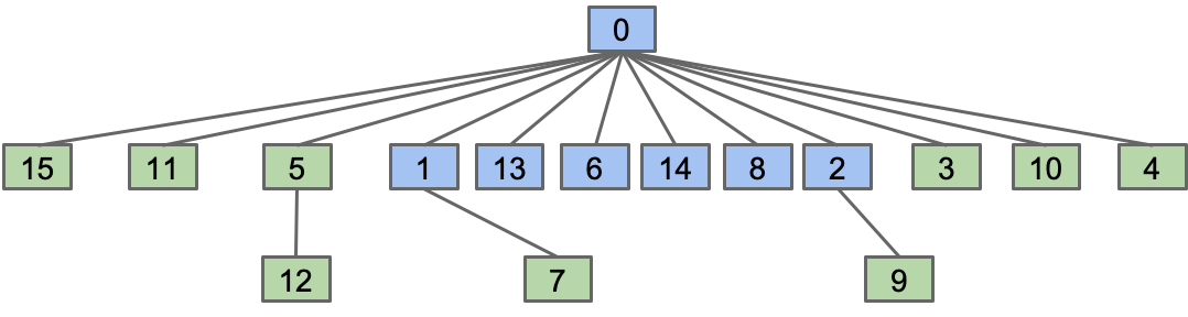
connected(0, 7):
    Does 0 == 7? No, so...
    If (connected(1, 7)) return true;
connected(1, 7):
    Does 1 == 7? No, so…
    If (connected(0, 7)) … ← Infinite loop.

How do we fix it?

Depth First Search

Basic idea is same as before, but visit each vertex at most once. [Demo]

def connected(s, t):
    marked[s] = True   # added
    if s == t:
        return True
    for v in neighbors_of(s):
        if not marked[v]  # added
            if connected(v, t):
                return True
    return False

Tree vs. Graph Traversals

Another example: DepthFirstPaths

Find a path from s to every other reachable vertex. [Demo]

def dfs(v):
    marked[v] = True
    for w in neighbors_of[v]:
        if not marked[w]:
            edgeTo[w] = v
            dfs(w)

This is called “DFS Preorder”. i.e., Action (setting edgeTo) is before DFS calls to neighbors. One valid DFS preorder for this graph: 012543678, equivalent to the order of dfs calls.

We could also do actions in DFS Postorder. i.e., Action is after DFS calls to neighbors. Example:

def dfs(s):
  marked[s] = True
  for w in neighbors_of[v]:
    if not marked[w]:
      dfs(w)
  print(s)

Results for dfs(0) would be: 347685210, equivalent to the order of dfs returns.

Just as there are many tree traversals, so too are there many graph traversals:

• DFS Preorder: 012543678 (dfs calls).
• DFS Postorder: 347685210 (dfs returns).
• BFS order: Act in order of distance from s.
  • BFS stands for “breadth first search”.
  • Analogous to “level order”. Search is wide, not deep.
  • 0 1 24 53 68 7

Summary

Graphs are a more general idea than a tree. A tree is a graph where there are no cycles and every vertex is connected. Graph problems vary widely in difficulty. Common tool for solving almost all graph problems is traversal. A traversal is an order in which you visit / act upon vertices.

• Tree traversals: Preorder, inorder, postorder, level order.
• Graph traversals: DFS preorder, DFS postorder, BFS.

By performing actions / setting instance variables during a graph (or tree) traversal, you can solve problems like s-t connectivity or path finding.

Graph Traversals and Implementations

Breadth First Search

Shortest Paths Challenge

Given the graph above, find the shortest path from s to all other vertices.

BFS Answer [Demo]

def bfs():
    fringe = deque([s])
    while fringe:
        v = fringe.popleft()
        for w in neighbors_of[v]:
            if not marked[w]:
                marked[w] = True
                edgeTo[w] = v
                #
            fringe.append(w)

Graph Representations

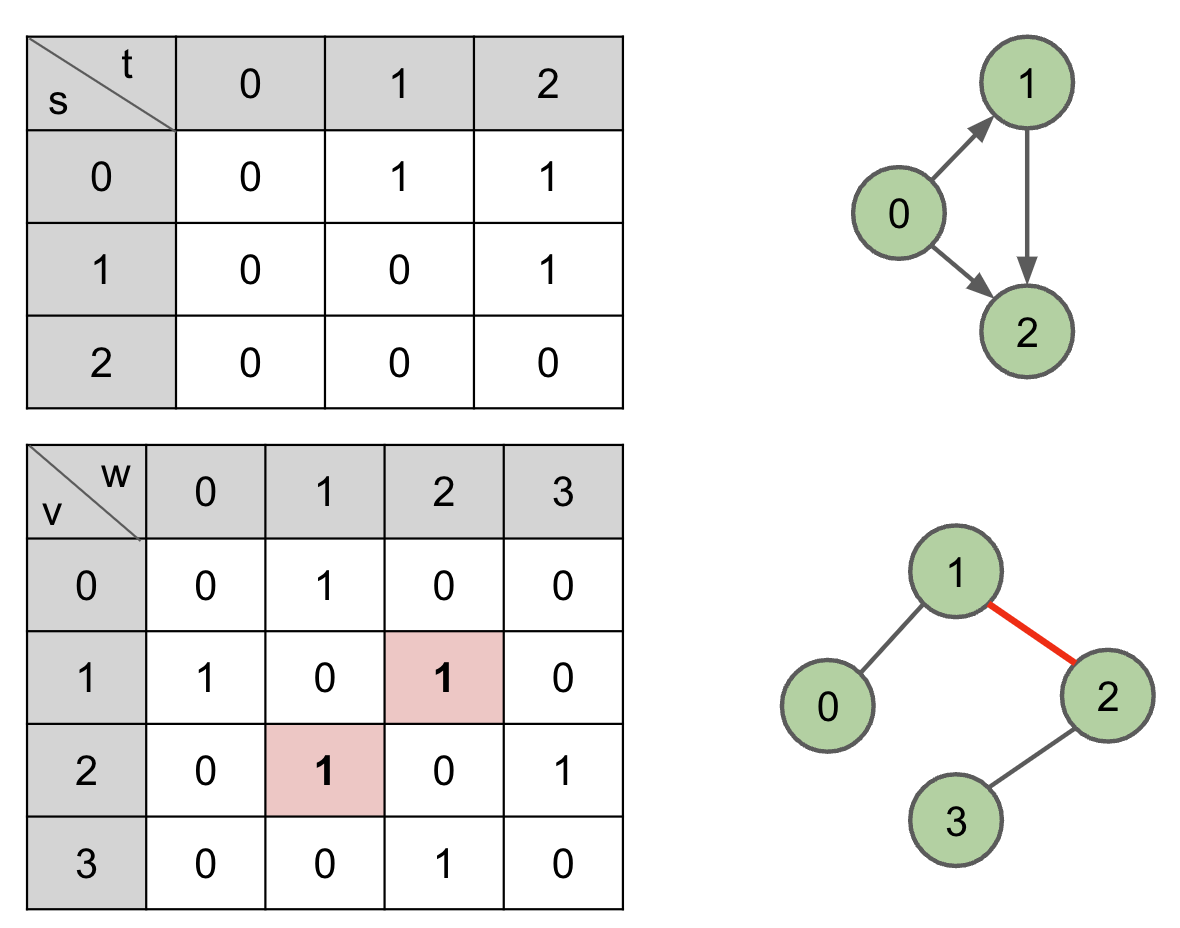
Adjacency Matrix

DFS, BFS Runtime: $O(V^2)$

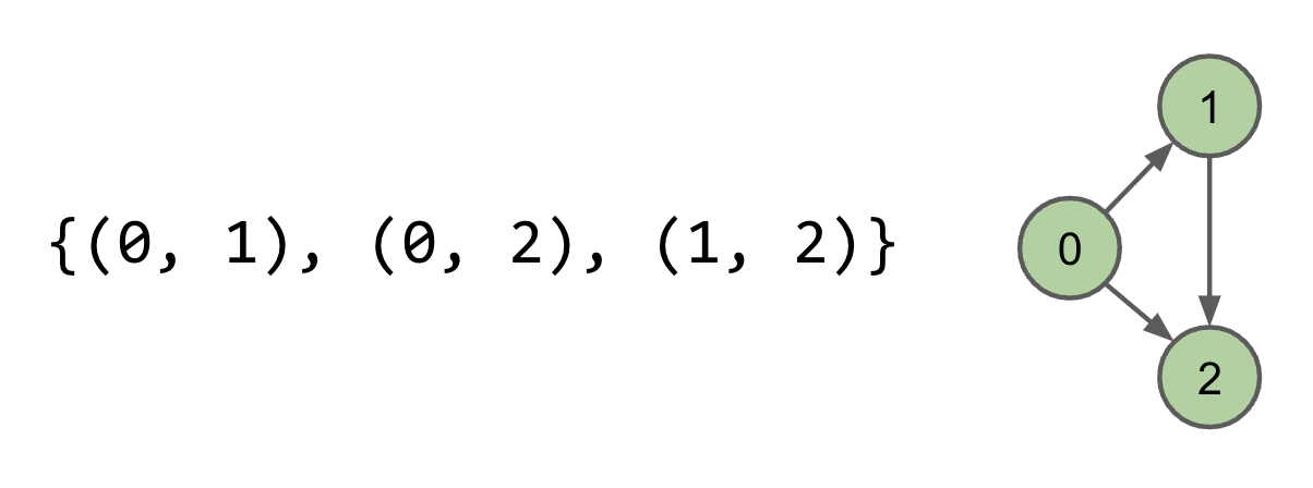
Edge Sets

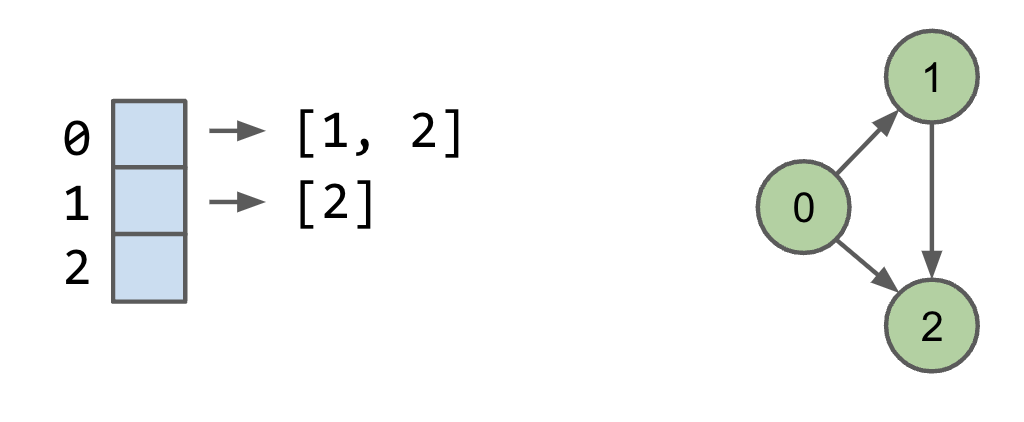
Adjacency Lists

Common approach: Maintain array of lists indexed by vertex number. Most popular approach for representing graphs. Efficient when graphs are “sparse” (not too many edges).

DFS, BFS Runtime: $O(V+E)$